Credit Risk Modeling

Introduction

One of the most exciting trends in FinTech innovation is the use of big data to simplify financial decision and provide comprehensive solution to its stakeholders. This is mainly due to large volumes of financial data that is available in recent times. Undoubtedly, one major area of concern in finance that has seen an unprecedented solution from leveraging big data with analytics is Credit Risk Management.

Credit Risk could simply be defined as the possibility of loss resulting from a borrower’s failure to repay a loan or meet contractual obligations on specified terms. Almost all financial institutions remain vulnerable to credit risk as far as lending forms an integral part of its services to the society. Managing Credit Risk has, therefore, become a top priority in the financial industry as firms need to protect themselves from loss of economic capital and bankruptcy.

Data

The data is provided by Home Credit, a service dedicated to provided lines of credit (loans) to the unbanked population. You can retreive the data here

There are 7 different sources of data:

• application_train/application_test: the main training and testing data with information about each loan application at Home Credit. Every loan has its own row and is identified by the feature SK_ID_CURR. The training application data comes with the TARGET indicating 0: the loan was repaid or 1: the loan was not repaid.
• bureau: data concerning client’s previous credits from other financial institutions. Each previous credit has its own row in bureau, but one loan in the application data can have multiple previous credits.
• bureau_balance: monthly data about the previous credits in bureau. Each row is one month of a previous credit, and a single previous credit can have multiple rows, one for each month of the credit length.
• previous_application: previous applications for loans at Home Credit of clients who have loans in the application data. Each current loan in the application data can have multiple previous loans. Each previous application has one row and is identified by the feature SK_ID_PREV.
• POS_CASH_BALANCE: monthly data about previous point of sale or cash loans clients have had with Home Credit. Each row is one month of a previous point of sale or cash loan, and a single previous loan can have many rows.
• credit_card_balance: monthly data about previous credit cards clients have had with Home Credit. Each row is one month of a credit card balance, and a single credit card can have many rows.
• installments_payment: payment history for previous loans at Home Credit. There is one row for every made payment and one row for every missed payment.

Determine Metric

Since we are trying tio determine the probability of default of a tarnsaction, it is a binary classification problem. There are several metrics that we can choose from

• accuracy
• precision
• Recall
• ROC/AUC

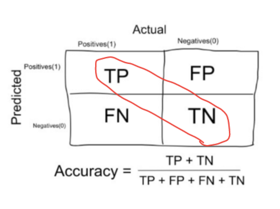
Accuracy in classification problems is the number of correct predictions made by the model over all kinds predictions made. Accuracy can be calculated as following:

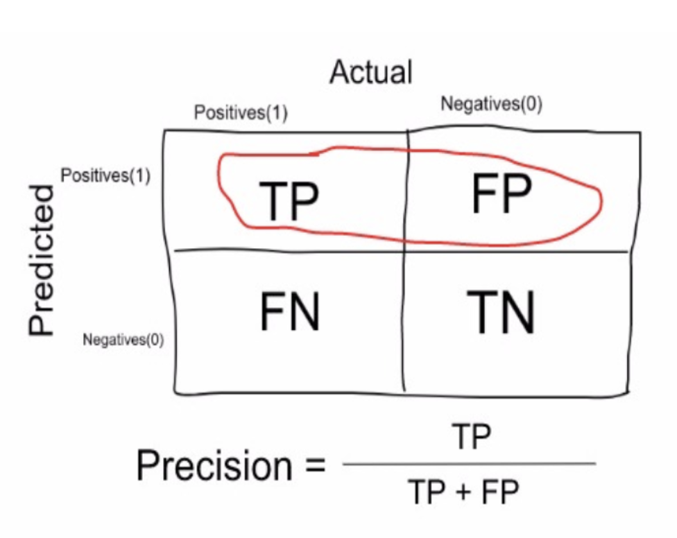
Precision is a measure that tells us what proportion of loans that we diagnosed as going default, actually defaulted. The predicted positives (People predicted as likely to default are TP and FP) and the people actually defaulted are TP.

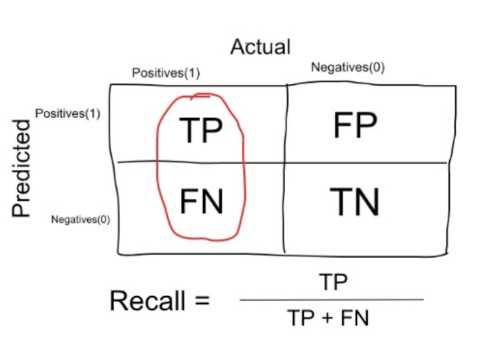
Recall is a measure that tells us what proportion of users that actually defaulted was diagnosed by the algorithm as going to default. The actual positives (People defaulted are TP and FN) and the people diagnosed by the model going to default are TP.

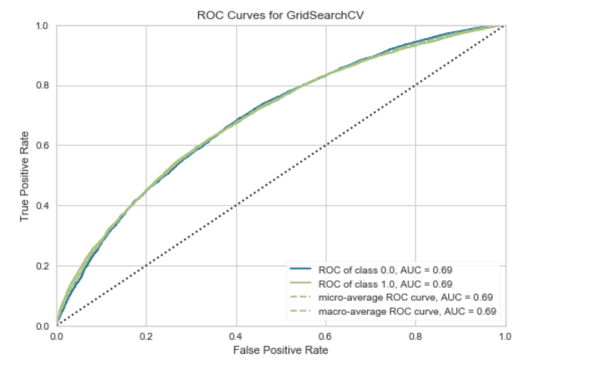
ROC It is a chart that visualizes the tradeoff between true positive rate (TPR) and false positive rate (FPR). Basically, for every threshold, we calculate TPR and FPR and plot it on one chart. Of course, the higher TPR and the lower FPR is for each threshold the better and so classifiers that have curves that are more top-left-side are better. n order to get one number that tells us how good our curve is, we can calculate the Area Under the ROC Curve, or ROC AUC score. The more top-left your curve is the higher the area and hence higher ROC AUC score.

Alternatively, it can be shown that ROC AUC score is equivalent to calculating the rank correlation between predictions and targets. From an interpretation standpoint, it is more useful because it tells us that this metric shows how good at ranking predictions your model is. It tells you what is the probability that a randomly chosen positive instance is ranked higher than a randomly chosen negative instance.

Since we care the ranking prediction which means we would rather people who are actually going to default should have higher likely hood than the people who are less likely to default. We will use AUC as our evaluation metrics.

Import data

we first import all libraries and read all the files

import pandas as pd
import numpy as np
import matplotlib.pyplot as plt
import seaborn as sns
import missingno as mn
import pandas_profiling as pp
import warnings
warnings.filterwarnings('ignore')
%matplotlib inline

application_train = pd.read_csv('application_train.csv')
application_test = pd.read_csv('application_test.csv')

Blind Machine Learning

I would first like to feed all numerical feature into a selection of models to see if it is even necessary to perform additional steps to mannually generate additional features.

def blind_ml_scores(X,y,metrics):
    scaler = StandardScaler()
    x = scaler.fit_transform(X)
    #x_test = scaler.transform(x_test)
    models = {'Dummy Classifier': DummyClassifier(strategy='prior'),
            'Logistic Regression' : LogisticRegression(),
              'Naive Bayes': BernoulliNB(),
              'Linear DIscriminant Analysis': LinearDiscriminantAnalysis(),
              'Neural Network': MLPClassifier(),
              'K Nearest Neighbor': KNeighborsClassifier(),
              'Random Forest':  RandomForestClassifier(),
              'Support Vector Machine': SVC(),
              'Gradient Boosting Tree': GradientBoostingClassifier()}
    scores = {}
    for name, clf in models.items():
        kfold = StratifiedKFold(n_splits=5,shuffle=True,random_state=3)
        s = cross_val_score(
            clf, x, y, scoring=metrics, cv=kfold,
        )
        scores[name+" "+metrics] = s.mean()
    return scores 
    
accuracy = blind_ml_scores(X,y,'accuracy')
f1 = blind_ml_scores(X,y,'f1')

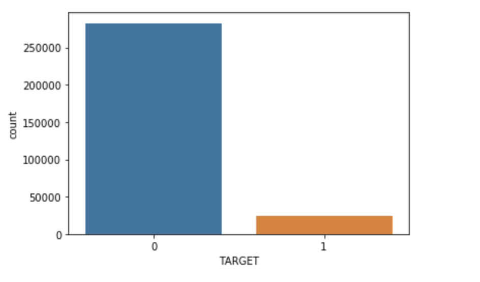
F1 score can be calculated as 2 (precisionrecall)/(precision+recall). One interesting aspect of the result is that the dummy classifier has reached 90% accuracy with 0 f1 score which shows that just looking at accuracy metric is not enough.

Exploratory analysis

categorical Variables

The target is what we are asked to predict: either a 0 for the loan was repaid on time, or a 1 indicating the client had payment difficulties. We can first examine the number of loans falling into each category.

check if education is a significant indicator of target variable

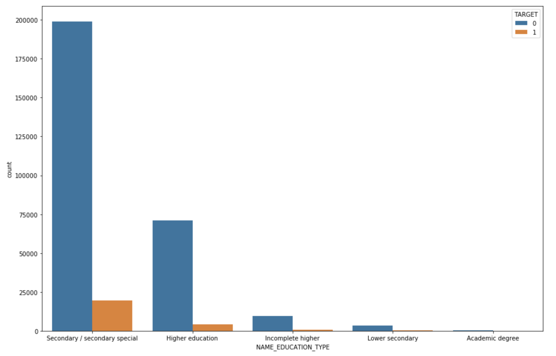
Most of the default comes from a secondary sepecial degree. Now Let’s check the occupation as an indicator.

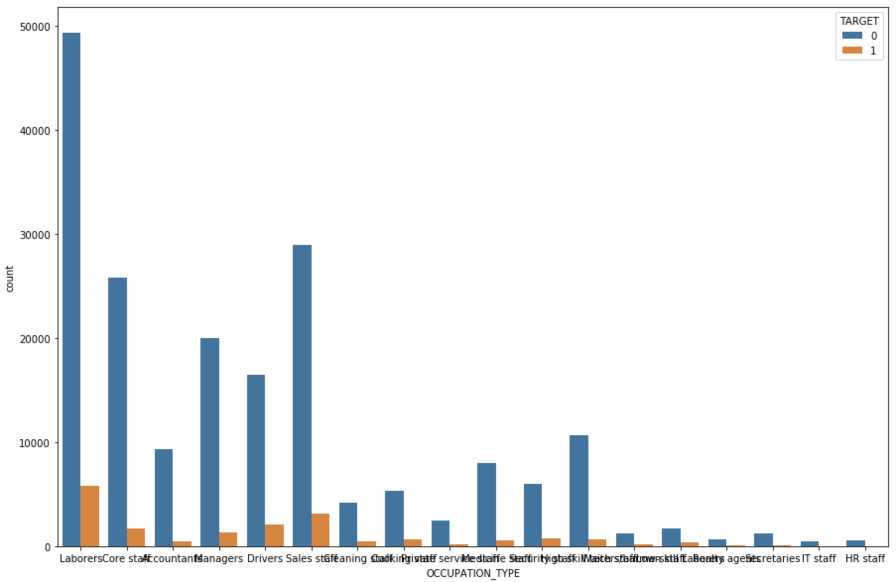
Most defaulted loan come from labor force.

Before we go any further, we need to deal with pesky categorical variables. A machine learning model unfortunately cannot deal with categorical variables (except for some models such as LightGBM). Therefore, we have to find a way to encode (represent) these variables as numbers before handing them off to the model. There are two main ways to carry out this process:

• Label encoding: assign each unique category in a categorical variable with an integer. No new columns are created. An example is shown below
• One-hot encoding: create a new column for each unique category in a categorical variable. Each observation recieves a 1 in the column for its corresponding category and a 0 in all other new columns.

The problem with label encoding is that it gives the categories an arbitrary ordering. The value assigned to each of the categories is random and does not reflect any inherent aspect of the category. Therefore, when we perform label encoding, the model might use the relative value of the feature to assign weights which is not what we want. If we only have two unique values for a categorical variable (such as Male/Female), then label encoding is fine, but for more than 2 unique categories, one-hot encoding is the safe option.

In this notebook, we will use Label Encoding for any categorical variables with only 2 categories and One-Hot Encoding for any categorical variables with more than 2 categories. This process may need to change as we get further into the project, but for now, we will see where this gets us.

Sample Imbalance

Imbalanced classifications pose a challenge for predictive modeling as most of the machine learning algorithms used for classification were designed around the assumption of an equal number of examples for each class. This results in models that have poor predictive performance, specifically for the minority class. This is a problem because typically, the minority class is more important and therefore the problem is more sensitive to classification errors for the minority class than the majority class.

These methods are often presented as great ways to balance the dataset before fitting a classifier on it. In a few words, these methods act on the dataset as follows:

• undersampling consists in sampling from the majority class in order to keep only a part of these points
• oversampling consists in replicating some points from the minority class in order to increase its cardinality
• generating synthetic data consists in creating new synthetic points from the minority class (see SMOTE method for example) to increase its cardinality

At this point, I would like to perform undersampling method since we have plenty samples.

def downsample(df,target_col):
    count_class_0, count_class_1 = df[target_col].value_counts()
    df_class_1 = df[df[target_col] == 1]
    df_class_0 = df[df[target_col] == 0]
    
    df_class_0_under = df_class_0.sample(count_class_1)
    df_under = pd.concat([df_class_0_under, df_class_1], axis=0,ignore_index=True)
    return df_under

Missing values

There are normally two ways to solve missing values which is imputation and removing data. We decide to simply allow user to specify a threshold. If the missing rate of a feature passed the threshold, we will drop this feature. However, there are also other methods listed below.

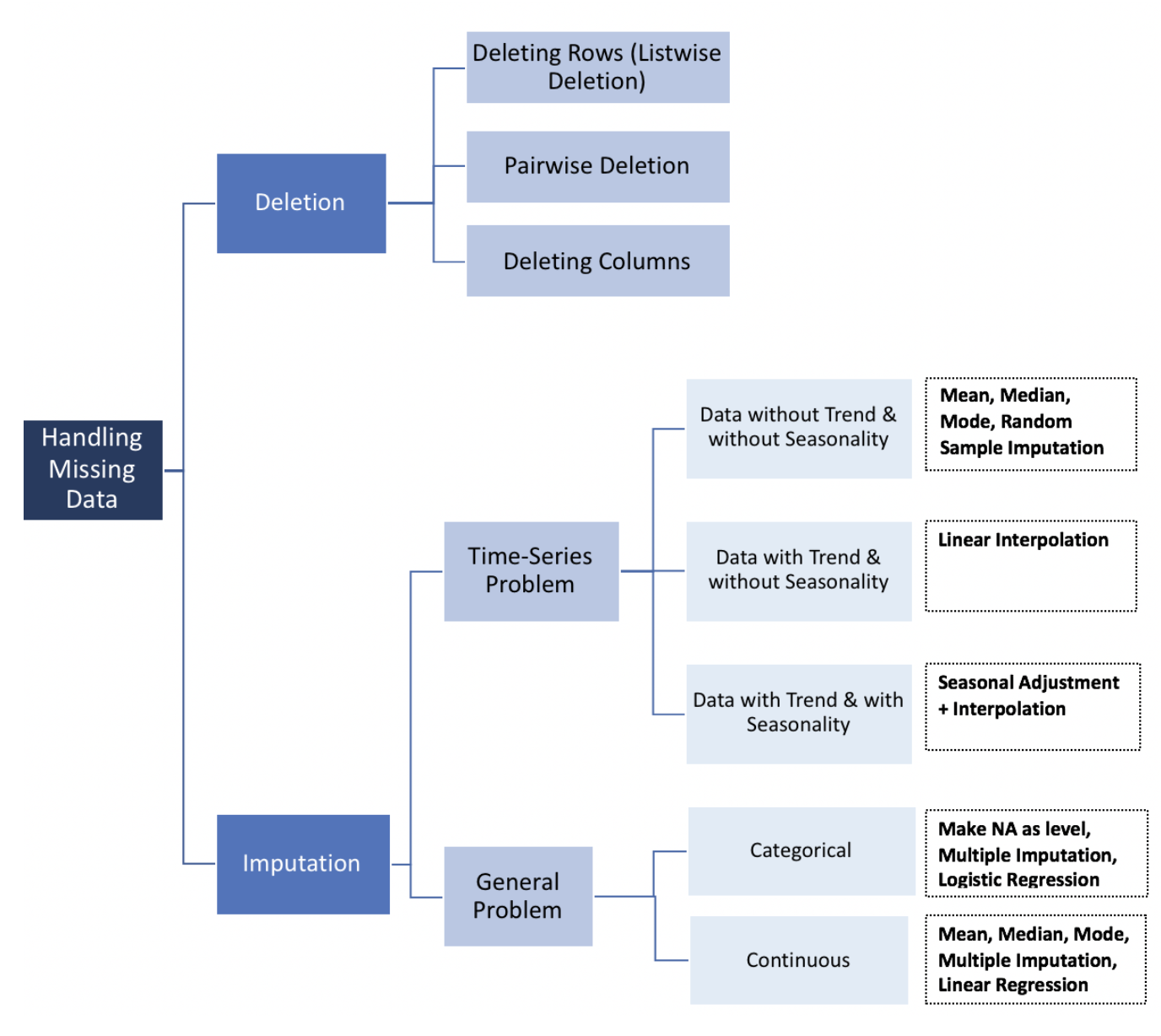
df = df.dropna(axis=1,how='any',thresh=int(0.7*len(temp)))

In this case, I choose the threshold to be 30%. After data cleaning, our dataset has 49,650 samples and 164 features.

Feature Selection

feature selection: choosing only the most important features or other methods of dimensionality reduction. Since there are 164 features within the dataset, will select the top 20 features with following methods:

• wrapper: search for well-perform features
  • RFE
• filter: select subset of feature based on their relationship with target variable
  • statistical method
    1. set a variance threshold, if the feature variance is less then the threshold, we will not use it. Other wise keep it. use VarianceThreshold.
    2. set correlation coefficient threshold, check the correlation coefficient with respect to target variable. less than threshold, we will discard. otherwise keep. use Person correlation
    3. use chi square test, set a chi square score threshold, select the top k feature with largest chi square statistics. larger chi square statistics means more relavant, use chi2 in sklearn. When two features are independent, the observed count is close to the expected count, thus we will have smaller Chi-Square value. So high Chi-Square value indicates that the hypothesis of independence is incorrect. In simple words, higher the Chi-Square value the feature is more dependent on the response and it can be selected for model training.
    4. use f test, set f score threshold. use f_classif in sklearn. f test is used to test if there is any difference between the variance of two variables. F Test is a statistical test used to compare between models and check if the difference is significant between the model. F-Test does a hypothesis testing model X and Y where X is a model created by just a constant and Y is the model created by a constant and a feature. The least square errors in both the models are compared and checks if the difference in errors between model X and Y are significant or introduced by chance.F-Test is useful in feature selection as we get to know the significance of each feature in improving the model.
  • feature importance method
    1. in sklearn use mutual_info_classif to calculate th mutual information between each feature and target variable, with higher mutual information, higher correlation.
• intrinsic: algorithm that perform automatic feature selection during training
  • decision Tree
  • L1/L2 regularization
  • in scikit learn use selectfrommodel to pick.

def feature_selection_rfe(df,target_col,numFeatures):
    temp=df.copy()
    X = temp.drop(target_col,axis=1).values
    y = temp[target_col].values
    models ={'dt': DecisionTreeClassifier(),
             'lr':LogisticRegression(),
             'nn':Perceptron(),
             'rf':RandomForestClassifier(),
             'gbm':GradientBoostingClassifier()
            }
    result = {}
    all_features = []
    frequency = {}
    #select all top 5 feature based on different model
    for name,clf in models.items():
        rfe = RFE(estimator=clf,n_features_to_select=5,step=1)
        rfe.fit(X,y)
        select_cols = []
        for i in range(X.shape[1]):
            if rfe.support_[i]:
                select_cols.append(temp.columns[i])
        result[name + ' selected features'] = select_cols
        #add all selected feature into a single list
        all_features.extend(select_cols)
    #calcualte each selected features frequency.  
    for classifier, features in result.items():
        for feature in features:
            frequency[feature] = all_features.count(feature)
    #select top 5 most appeared features
    #sorted_frequency = sorted(frequency.items(), key=lambda kv: -kv[1])
    features_sorted = heapq.nlargest(numFeatures, frequency) 
    return sorted_frequency

def feature_selection_variance(df,target_col,threshold):
    """select the feature based on variance threshold
    Parameters
    ----------
    df: original dataframe. pd.Dataframe
    target_col: target variable. string
    threshold: the variance threshold. between 0 and 1. float
    
    Return:
    X_new: selected new feature. np.arrray
    """
    X = df.drop(target_col,axis=1)
    thresholder = VarianceThreshold(threshold)
    X_new = thresholder.fit_transform(X)
    cols = thresholder.get_support(indices=True)
    features_df_new = df.iloc[:,cols]
    return X_new

def feature_selection_correlation(df,target_col,k):
    high_corr_features = list(df.corr()[[target_col]].nlargest(k,columns=target_col).index)[1:] + target_col
    return df[high_corr_features]
    
def feature_selection_statistic(df,target_col,numFeatures,method='chi2'):
    """based on test statistic to determine the features. higher statistics 
                             means higher correlation toward target variable
    Parameters
    ----------
    df: original dataframe. pd.Dataframe
    target_col: target variable. string
    method: select from "chi2" (chi square test),"f_class_if" (f test), "mutual_info_classif" (mutual information)
    
    Return:
    X_new: selected new feature. np.arrray
    """
    X = df.drop(target_col,axis=1)
    y = df[target_col]
    selector = None
    if method == 'chi2':
        selector = SelectKBest(chi2,k=numFeatures)
        X_new = selector.fit_transform(X,y)
    elif method=='f_class_if':
        selector = SelectKBest(f_classif,k=numFeatures)
        X_new = selector.fit_transform(X,y)
    elif method == 'mutual_info_classif':
        selector = SelectKBest(mutual_info_classif,k=numFeatures)
        X_new = selector.fit_transform(X,y)
    
    cols = selector.get_support(indices=True) + target_col
    features_df_new = df.iloc[:,cols]
    return features_df_new
    #return X_new

def feature_selection_model(df,target_col):
    """select features based on L1 based model and tree based model
    Parameter
    ---------
    df: original dataframe. pd.Dataframe
    target_col: target variable. string
    
    Return
    ------
    X_new_table: each model and its corresponding feature selection result. dictionary
    """
    X = df.drop(target_col,axis=1)
    y = df[target_col]
    #With SVMs and logistic-regression, the parameter C controls the sparsity: the smaller C the fewer features selected. 
    #With Lasso, the higher the alpha parameter, the fewer features selected
    X_new_table = {}
    models = {
        #L1 based feature selection
        'Logistic_Regression': LogisticRegression(penalty='l1',C=0.1,solver='liblinear'),
        'Linear_SVC' : LinearSVC(penalty='l1',C=0.1,dual=False),
        #Tree based feature selection
        'DecisionTree_Classifier': DecisionTreeClassifier(),
        "RandomForest_Classifier": RandomForestClassifier(),
        'ExtraTree_Classifier': ExtraTreesClassifier()
    }
    for name, estimator in models.items():
        selector = SelectFromModel(estimator,threshold='median')
        X_new = selector.fit_transform(X,y)
        cols = selector.get_support(indices=True)
        features_df_new = df.iloc[:,cols]
        X_new_table[name + '_X_new'] = X_new
    return X_new_table

#select feature based on variance thrshold
X_variance_select = feature_selection_variance(temp,'TARGET',0.2)
# select feature based on correlation threshold
X_corr_select = feature_selection_correlation(temp,'TARGET',21)
# select feature based on f score threshold
X_f_select = feature_selection_statistic(temp,'TARGET',20,'f_class_if')
X_mutual_select = feature_selection_statistic(temp,'TARGET',20,'mutual_info_classif')
#select feature based on model built in feature importance
X_model_tables = feature_selection_model(temp,"TARGET")

Outlier detection

One problem we always want to be on the lookout for when doing EDA is anomalies within the data. These may be due to mis-typed numbers, errors in measuring equipment, or they could be valid but extreme measurements. One way is to use the describe method.

df['DAYS_EMPLOYED'].describe()

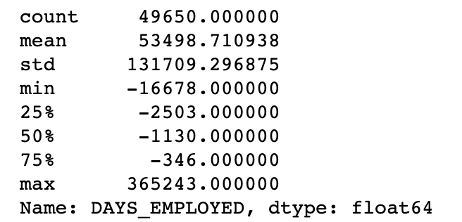
It is impossible to be emoployeed over 365000 days which is over 1000 years. The anomaly is also consist 15% of our data.

Feature engineering

Feature engineering refers to a geneal process and can involve both feature construction: adding new features from the existing data, and There are many techniques we can use to both create features and select features.

In order to better generate significant indicator, I have attempt to generate the following features:

• CREDIT_INCOME_PERCENT: the percentage of the credit amount relative to a client’s income
• ANNUITY_INCOME_PERCENT: the percentage of the loan annuity relative to a client’s income
• CREDIT_TERM: the length of the payment in months (since the annuity is the monthly amount due
• DAYS_EMPLOYED_PERCENT: the percentage of the days employed relative to the client’s age

app_train_domain = temp.copy()

app_train_domain['CREDIT_INCOME_PERCENT'] = app_train_domain['AMT_CREDIT'] / app_train_domain['AMT_INCOME_TOTAL']
app_train_domain['ANNUITY_INCOME_PERCENT'] = app_train_domain['AMT_ANNUITY'] / app_train_domain['AMT_INCOME_TOTAL']
app_train_domain['CREDIT_TERM'] = app_train_domain['AMT_ANNUITY'] / app_train_domain['AMT_CREDIT']
app_train_domain['DAYS_EMPLOYED_PERCENT'] = app_train_domain['DAYS_EMPLOYED'] / app_train_domain['DAYS_BIRTH']

fig = plt.figure(figsize = (12, 20))
# iterate through the new features
for i, feature in enumerate(['CREDIT_INCOME_PERCENT', 'ANNUITY_INCOME_PERCENT', 'CREDIT_TERM', 'DAYS_EMPLOYED_PERCENT']):
    
    # create a new subplot for each source
    plt.subplot(4, 1, i + 1)
    # plot repaid loans
    sns.kdeplot(app_train_domain.loc[app_train_domain['TARGET'] == 0, feature], label = 'target == 0')
    # plot loans that were not repaid
    sns.kdeplot(app_train_domain.loc[app_train_domain['TARGET'] == 1, feature], label = 'target == 1')
    
    # Label the plots
    plt.title('Distribution of %s by Target Value' % feature)
    plt.xlabel('%s' % feature); plt.ylabel('Density');
    
plt.tight_layout(h_pad = 2.5)
plt.savefig('feature_engineering.png')

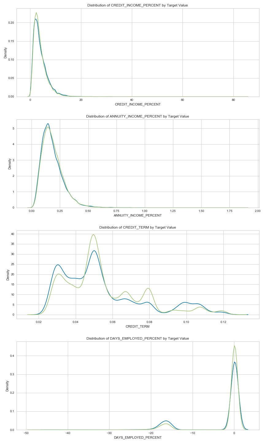
There appears to have no visually obvious cutoff threshold. Perhaps Machine Learning Models can help us out.

Modeling

We have selected several models and we will use sklearn package.

from sklearn.linear_model import (
    LogisticRegression,
)
from sklearn.tree import (
    DecisionTreeClassifier,
)
from sklearn.neighbors import (
    KNeighborsClassifier,
)
from sklearn.naive_bayes import (
    GaussianNB,
)
from sklearn.svm import (
    SVC,
)
from sklearn.ensemble import (
    RandomForestClassifier,
)
import xgboost

models = [    
    DummyClassifier,
    LogisticRegression,
    DecisionTreeClassifier,
    KNeighborsClassifier,
    GaussianNB,
    SVC,
    RandomForestClassifier,
    xgboost.XGBRFClassifier,
]

for model in models:
    cls = model()
    kfold = model_selection.KFold(
        n_splits=10, 
        shuffle=True,
        random_state=123,
    )
    s = model_selection.cross_val_score(
        cls, X, y, scoring='roc_auc', cv=kfold,
    )
    print(
        f'{model.__name__:22} AUC:'
        f'{s.mean():.3f} STD: {s.std():.2f}'
    )

From the result, the xgboost classifier has the highest AUC score of 0.686. After we have added engineered feature, the AUC score are still 0.686 which does not improve.

Hyparameter tunning

clf_ = xgboost.XGBRFClassifier()
params = {
    'min_child_weight': [1, 5, 10],
    'gamma': [0, 0.5, 1, 1.5, 2, 5],
    'colsample_bytree': [0.6, 0.8, 1.0],
    'max_depth': [4, 5, 6, 7],
}
clf = model_selection.GridSearchCV(
    clf_, params, n_jobs=-1, 
).fit(X_train, y_train)
clf_best = clf.best_estimators_
roc_auc_score(
    y_test, clf_best.predict(X_test)
)

After tunning, the xgboost classifier has reached AUC score of 0.694.

Model Evaluation

• Confusion Matrix

  from yellowbrick.classifier import ConfusionMatrix
  cm_viz = ConfusionMatrix(clf, classes=['non-default', 'default'])
  cm_viz.fit(X_train, y_train)
  cm_viz.score(X_test, y_test)
  cm_viz.show();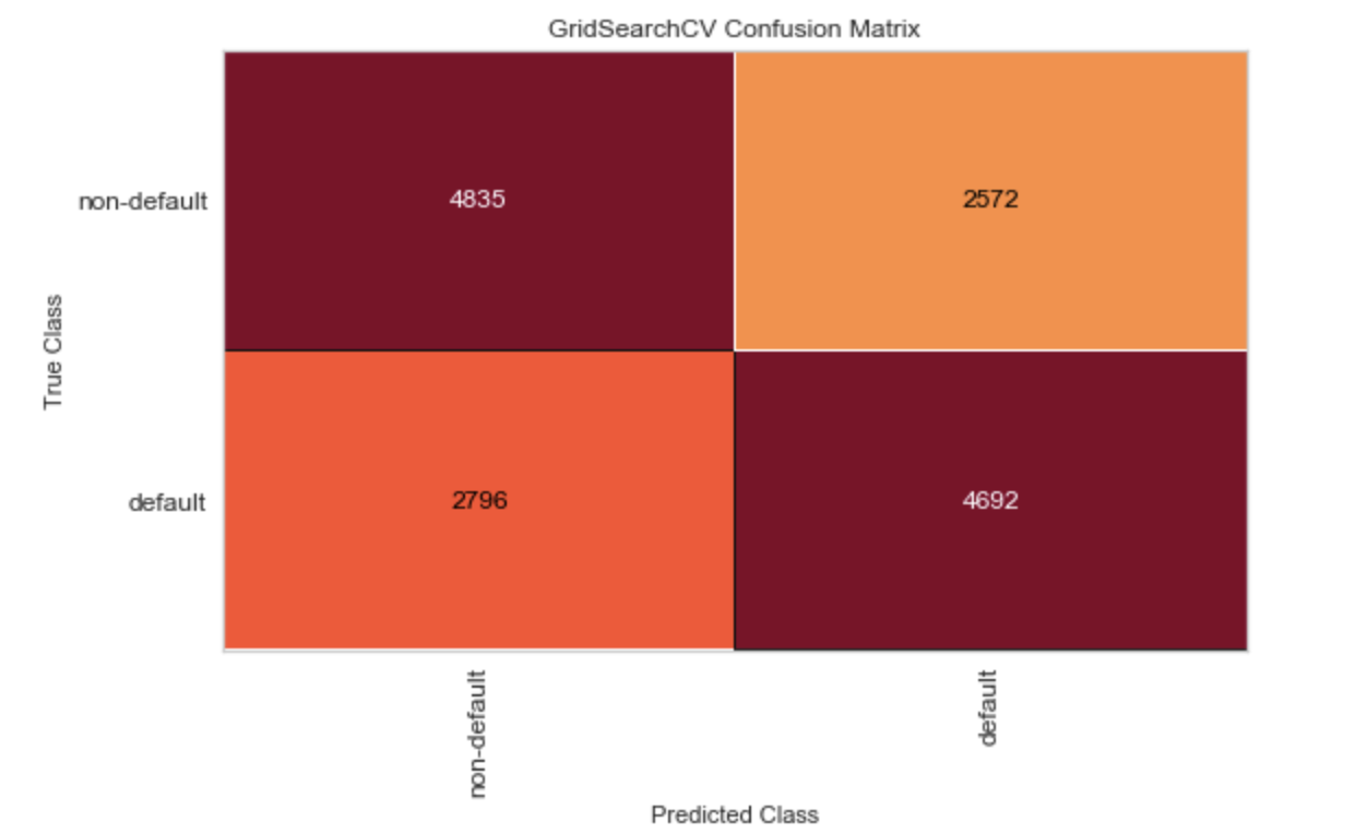
  

  

  The above result has shown that the classifier did equally bad job prredicting default and non default jobs.

• ROC curve

  

• Precision-recall curve

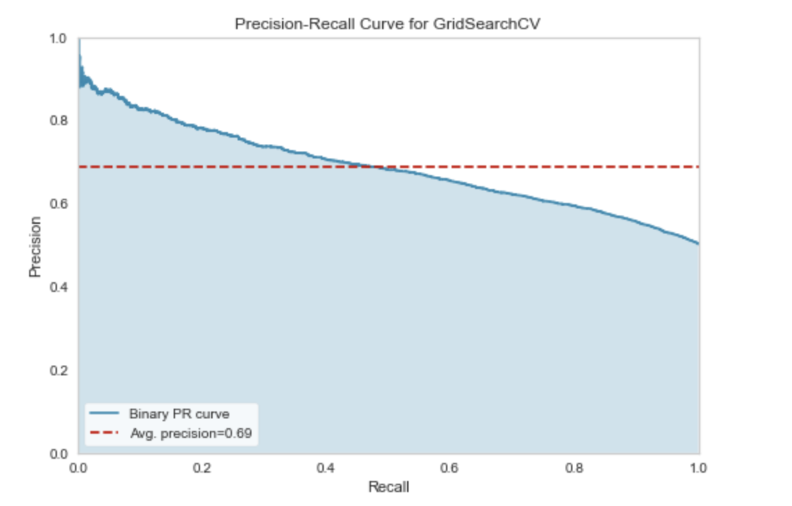
The AUC score is 0.69. Perhaps with additional feature engineering from the dataset, the AUC score may improve.

Model Interpretation

As a simple method to see which variables are the most relevant, we can look at the feature importances of the random forest. Given the correlations we saw in the exploratory data analysis, we should expect that the most important features are the EXT_SOURCE and the DAYS_BIRTH. We may use these feature importances as a method of dimensionality reduction in future work.

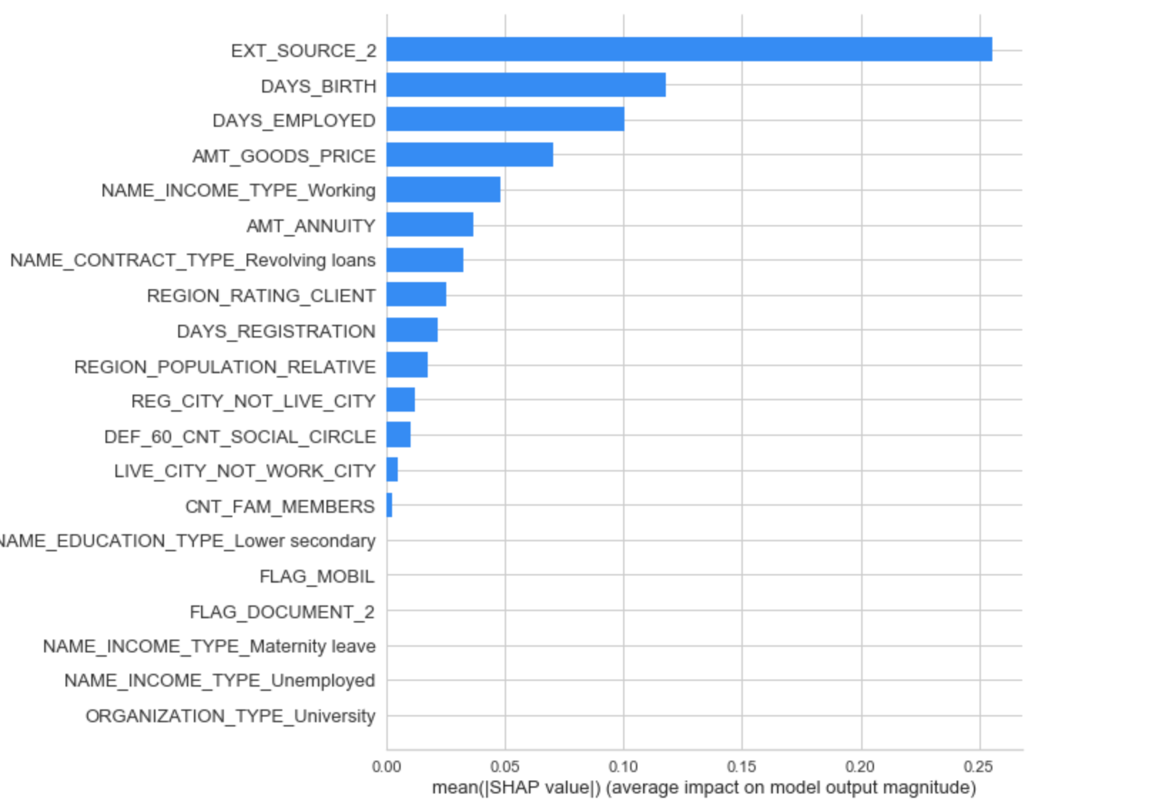
As expected, the most important features are those dealing with EXT_SOURCE and DAYS_BIRTH. We see that there are only a handful of features with a significant importance to the model, which suggests we may be able to drop many of the features without a decrease in performance (and we may even see an increase in performance.)

Shapley Additive exPlanations (SHAP)

A concept from game theory - Nobel Prize in Economics 2012

In the ML context, the game is prediction of an instance, each player is a feature, coalitions are subsets of features, and the game payoff is the difference in predicted value for an instance and the mean prediction (i.e. null model with no features used in prediction).

The Shapley value is given by the formula

Shapley Additive exPlanations. Note that the sum of Shapley values for all features is the same as the difference between the predicted value of the full model (with all features) and the null model (with no features). So the Shapley values provide an additive measure of feature importance. In fact, we have a simple linear model that explains the contributions of each feature.

• Note 1: The prediction is for each instance (observation), so this is a local interpretation. However, we can average over all observations to get a global value.
• Note 2: There are 2𝑛2n possible coalitions of 𝑛n features, so exact calculation of the Shapley values as illustrated is not feasible in practice. See the reference book for details of how calculations are done in practice.
• Note 3: Since Shapley values are additive, we can just add them up over different ML models, making it useful for ensembles.
• Note 4: Strictly, the calculation we show is known as kernelSHAP. There are variants for different algorithms that are faster such as treeSHAP, but the essential concept is the same.
• Note 5: The Shapeley values quantify the contributions of a feature when it is added to a coalition. This measures something different from the permutation feature importance, which assesses the loss in predictive ability when a feature is removed from the feature set.

shap value summary plot

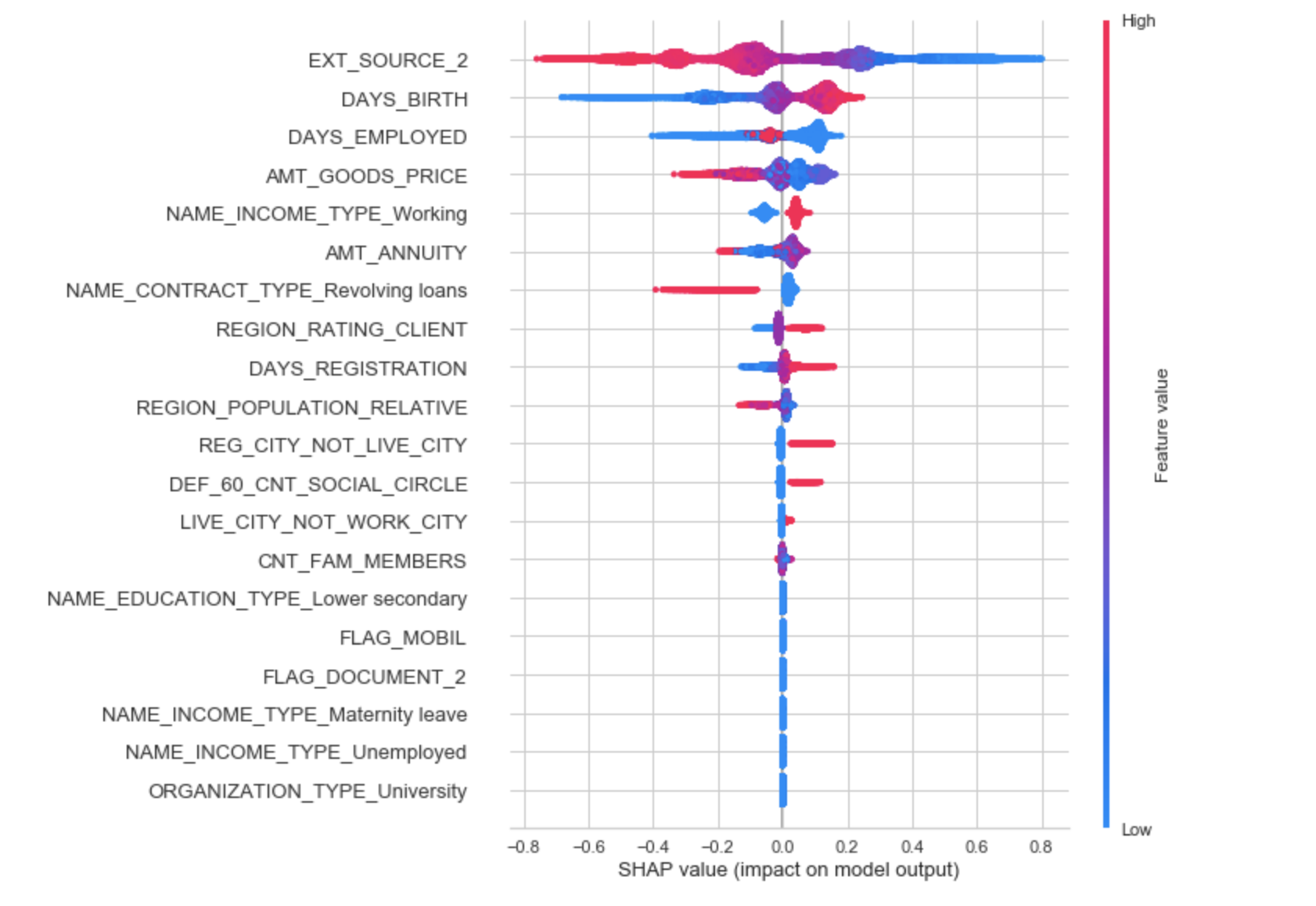
This shows the jittered Shapley values (in probability space) for all instances for each feature. An instance to the right of the vertical line (null model) means that the model predicts a higher probability of survival than the null model. If a point is on the right and is red, it means that for that instance, a high value of that feature predicts a higher probability of survival.

For example, EXT_SOURCE_2 shows that if you have a high value your probability of default is increased. Similarly, lower score predicts lower default probability.

Conclusion

In this notebook, We first made sure to understand the data, our task, and the metric. Then, we performed a fairly simple EDA to try and identify relationships, trends, or anomalies that may help our modeling. Along the way, we performed necessary preprocessing steps such as encoding categorical variables, imputing missing values, and scaling features to a range. Then, we constructed new features out of the existing data to see if doing so could help our model.

Once the data exploration, data preparation, and feature engineering was complete, we select a baseline model upon which we hope to improve. Then we tune the hyperparameters of the model to beat our first score. We also carried out an experiment to determine the effect of adding the engineering variables.

Interesting findings:

1. Current benchmark model has AUC score of 0.69
2. The top indicator of user default probability are age of user, user employment length, Their employment type and so on
3. Mannually Engineered feature such as credit_income_percent, annuity_income_percent, credit_term, days_employed_percent are not useful to improve the model’s AUC score. Because Some features may contains the same confounding varaible as engineered features.