Home_price

Introduction

Housing price are an an important Reflection of the economy, and housing prices ranges are of great interest for both buyers and sellers. In this project, house price index will be predicted given serveral indicator variables. The goal of this project is to create a regression model that are able to estimate the house index given the features and provide any interesting business insight within the dataset

Data Acquisition

This dataset is from Dr. Jimmie Lenz. The project aims to apply various python tools to get a visual understanding of the data and clean it to make it ready to apply machine learning algorithm. The dataset can be found here.

Data Cleaning

The original dataset is quite messy. There are 19 different features. However, most of the features are only labeling the data source and logged date. There are total 7 valuable variables

Independent variable:

• Cost index
• population
• Consumer price index
• long rate
• CPI annual
• Nominal home price index

dependent variable

• Real Home index

Data Exploratory analysis

# visualization of the trend of indexs
fig,ax = plt.subplots(figsize=(15,10))
origin_df.plot.line(x='home_index_date',y='real_home_index',ax=ax,label = 'real_home_index')
origin_df.plot.line(x='home_index_date',y='real_cost_index',ax=ax,label = 'real_cost_index')
origin_df.plot.line(x='home_index_date',y='population',ax=ax,label = 'population')
origin_df.plot.line(x='home_index_date',y='long_rate',ax=ax,label = 'long_rate')
origin_df.plot.line(x='home_index_date',y='cpi_annual',ax=ax,label = 'cpi_annual')
ax.set_xlabel('year')
ax.set_ylabel('index')
ax.set_title('yearly index trend')
plt.tight_layout()

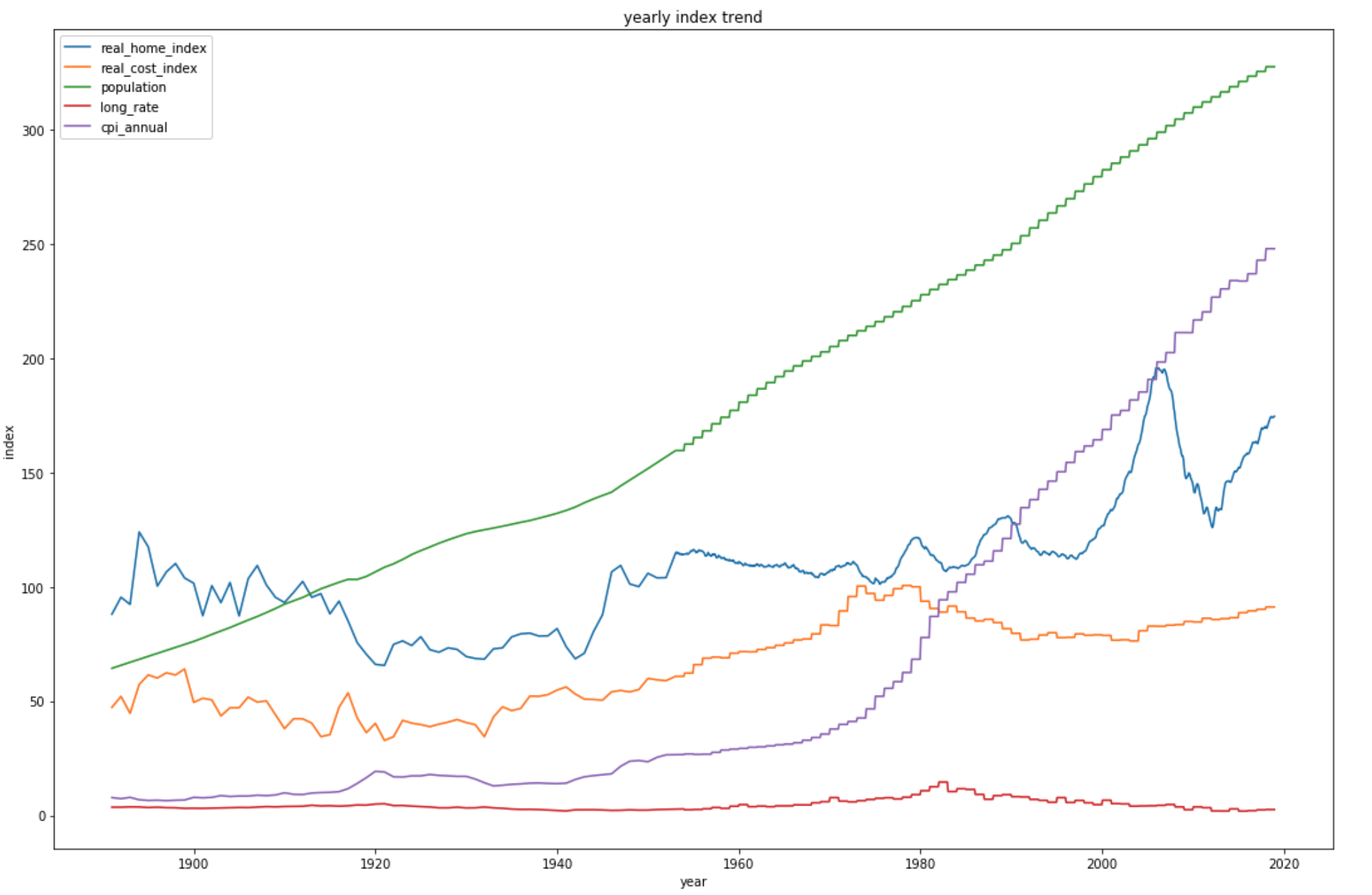
From the plot above, we can clearly see that home index, cost index, population and annual CPI are all increasing. However, the long rate stays relative constant.

The time sampling rate in this dataset is different

• the observation from 1890 to1952 are sampled on yearly bases
• the observation from 1953 to 2019 are sampled on monthly bases

There are two solution to the above issue:

1. downsample the data after 1953 to yearly bases and combine both parts and perform regression analysis
2. upsample the data befre 1952 to monthly baeses and combine both parts and perform regression analysis

downsample dataset approach

def downsample(original_df):
    '''downsample the dataframe from monthly bases into yearly bases
    Parameters
    ----------
    original_df: original dataframe. Pandas.Dataframe
    
    Return
    ------
    df: downsampled dataframe. Pandas.Dataframe
    '''
    
    df = origin_df
    df1 = df[df['home_index_date'] <= 1952]
    df2 = df[df['home_index_date'] > 1952]
    df2['year'],df2['day'] = df['home_index_date'].divmod(1)
    df2  = df2.groupby('year').min().reset_index()
    df2 = df2.drop(['home_index_date','day'],axis=1)
    df2.columns = ['home_index_date', 'real_home_index', 'real_cost_index', 'population','long_rate','cpi_annual']
    df = pd.concat([df1,df2],ignore_index=True)
    
    return df

after running the above program, there are total 128 observations within this dataset. In order to fit a linear regression model on the dataset, I also have to check the assumption for linear regression

• Linearity: The relationship between X and the mean of Y is linear
• Homoscedasticity: The variance of residual is the same for any value of X
• Independence: Observations are independent of each other
• Normality: For any fixed value of X, the residual error is normally distributed and additive.

I choose to use visualization method to test the linearity, homoscedasticity, normality. I also use Person Correlation coefficient method to verify the independence of our features.

def assumption_test(model,y):
    '''visualization of fitted value vs observed, residual vs fitted value, residual kernal density plot to exame the 
        assumption of linear regression
    Parameters
    ----------
    model: the linear regression model that I intend to test. statsmodel.models
    y: the observation ('home index')
    
    Return
    ------
    None
    '''
    fitted_values = model.predict()
    resids = model.resid
    
    fig, ax = plt.subplots(1,3,figsize=(16,8))
    #Linearity check
    sns.regplot(x=fitted_values,y=y,lowess=True,ax=ax[0])
    ax[0].set_title('fitted value vs observed')
    ax[0].set(xlabel='fitted value',ylabel='observed')
    
    #homoscedasticity check
    sns.regplot(x=fitted_values, y=resids, lowess=True, ax=ax[1], line_kws={'color': 'red'})
    ax[1].set_title('Residuals vs. fitted Values', fontsize=16)
    ax[1].set(xlabel='fitted value', ylabel='Residuals')
    
    #normality check
    sns.kdeplot(resids,ax=ax[2])
    ax[2].set_title('residual kde plot')
    ax[2].set(ylabel='density',xlabel='residual')

Each plot above corresponds to a assumption test for linear regression. Since there is only 128 observations as total samples. I choose to use the first 2/3 of the total samples (84) as training dataset and the rest of dataset is as testing dataset (The dataset is sorted in chronological order.)

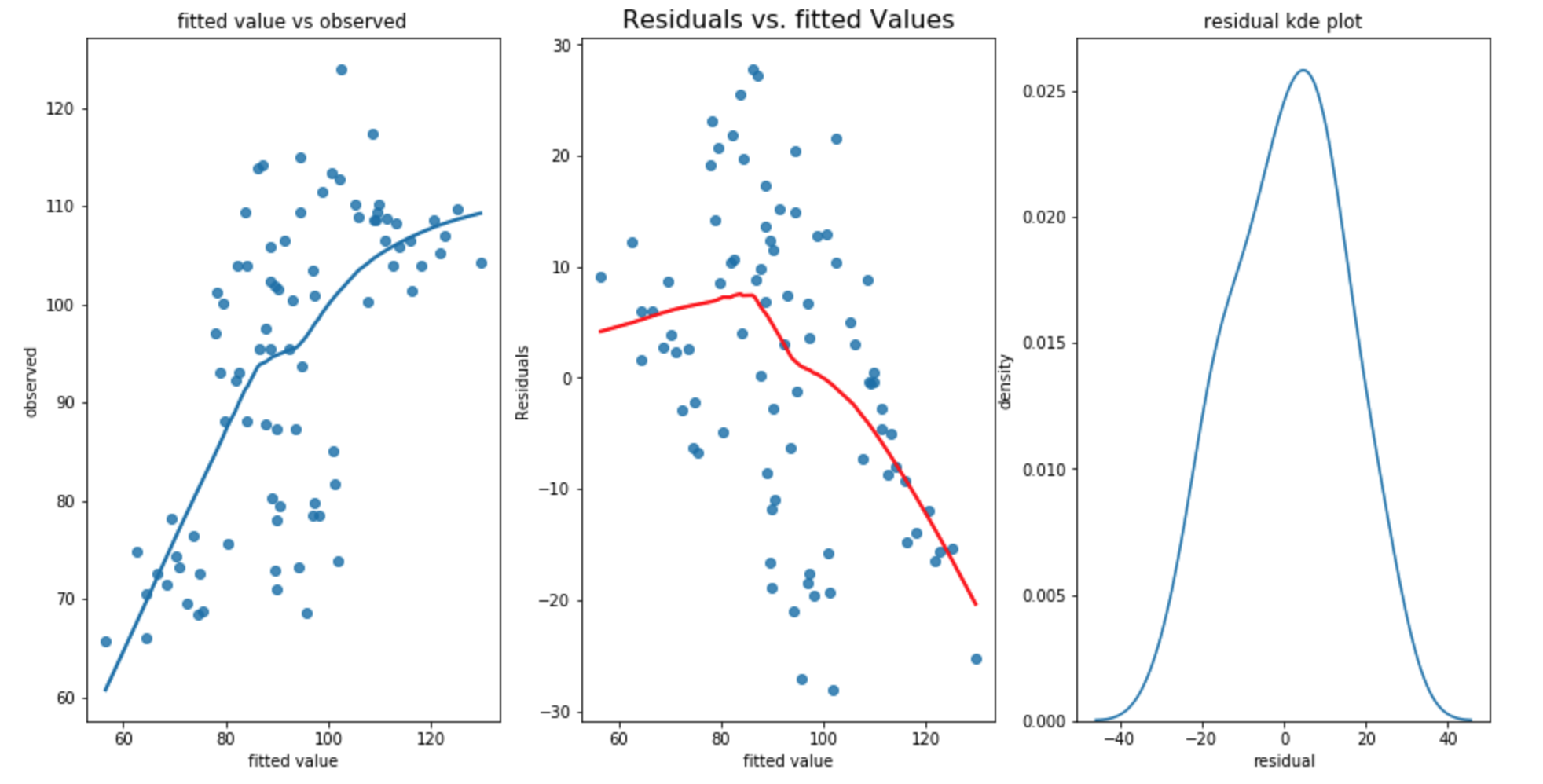
• the fitted value vs observation plot shows that observation value may not increased as fast as fitted value. it shows that the linearity may not be satisfied
• the residual vs fitted plot also shows that the residual are mostly positive when fitted value is small. However, some of the residual are negative and some residuals are positive when fitted value is large. Thus, the relationship doesn’t appear to be linear. In addition, the residual is not constant 0 and the variance appears to decrease as fitted value increased. The homoscedasticity is not satisified.
• the residual kernal density plot appears to be normal. the normality assumption is satisfied.

In order to fully understand the linear regression residual, I also plot ACF and perform a Durbin Watson test to test the stationarity of the residual. The Durbin Watson statistic provides a test for significant residual autocorrelation at lag 1. The statistic is approximately equal to 2*(1-a), where a is the lag 1 residual autocorrelation. The test statistic resides in the default summary out of statsmodel’s regression. some notes on the Durbin-Watson test:

• the test statistics alwasys has a value between 0 and 4
• value of 2 means that there is no autocorrelation in the sample
• values < 2 indicate positive autocorrelation, values > 2 indicate negative autocorrelation

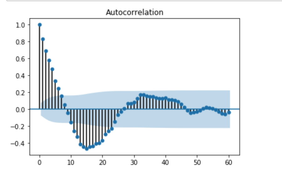
We can clearly see there is a autocorrelation when lag is smaller than 8. In addition, The Durbin Watson test statistic is 0.314 which means there is positive autocorrelation.

I have also calculate the Person Correlation among all the features and visualized in seaborn heatmaps.

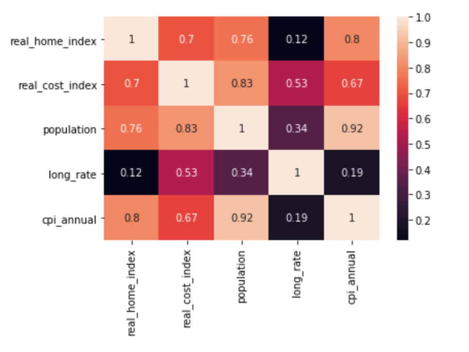
The threshold to determine the highly correlation between two variables are 0.8. From the heatmap, I can arrive the conclusion that populaton is highly correlate with cpi_annual. It may cause overfitting issue in Linear Regression

Potential solution

• Linearity:
  • Non-linear transformation to dependent/independent variable (square, log)
  • add extra features
• Homoscedasticity:
  • log transformation of the dependent variable
  • stationarize the series value (differencing, exponential smoothing)
  • in case of minor positive autocorrelation, there may be some room to fine tune the model, for example, adding the lags of the dependent/independent variables
  • capture the seasonal components
  • include a linear trend term in case of consistent increasing/decreasing pattern in the residual
• independence:
  • Perform feature selection
  • Perform PCA to reduce the feature to small set of uncorrelated component
• normality:
  • so far the residual appears to be normal

feature engineering

1. One of the potential solution for homoscedasticity is to generate lagged features. Model as the following equation:

   $y_t = \beta_0 + \beta_1 * x + \beta_2*y_{t-1} + \beta_3* x_{t-1} + \epsilon$

def add_features(data,n_in,dropnan):
    '''create lagged feature 
    
    Parameters
    ----------
    data: target timeseries data. pandas.Dataframe
    n_in: number of lag observations as input between 1 and len(data). float 
    dropna: wheather or not to drop the NaN values. Boolean 
    
    
    Returns
    -------
    df: new Pandas dataframe for supervised machine learning
    '''
    if isinstance(data,pd.Series):
        df = pd.DataFrame(data)
    elif isinstance(data,pd.DataFrame):
        df = data
    new_cols = [df]
    #lag all the columns in df
    for i in range(1,n_in+1):
        temp = df.shift(i)
        temp.columns = temp.columns + '_lag_' + str(i)
        temp.drop('home_index_date_lag_'+str(i),axis=1,inplace=True)
        new_cols.append(temp)
    
    new_df = pd.concat(new_cols,axis=1)
    
    if dropnan:
        new_df = new_df.dropna()
    return new_df

Since there are only 128 observations, it is best practice to not have over 10 features. Thus, I decide to use Random Forest to pick the top 10 most important features.

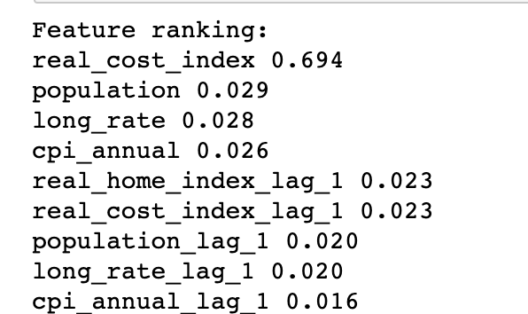
Random Forest model has selected all original feature and its lagged value as the most important features. I decide to build a linear regression model on selected feature with data from 1890 to 2008 (reserve the last 10 years data as test data). I also decide to use Root Mean Squared Error as our evaluation metrics.

from sklearn.metrics import mean_squared_error
rmse_test = np.sqrt(mean_squared_error(y_test,y_pred))
rmse_train = np.sqrt(mean_squared_error(y_train,lr.predict(x_train)))
std = np.std(y_test)
print("RMSE for training dataset is %.3f, RMSE for test dataset is %.3f and standard deviation of test dataset is %.3f"
      %(rmse_train,rmse_test,std))

RMSE for training dataset is 6.132, RMSE for test dataset is 9.085 and standard deviation of test dataset is 13.967. The Durbain Watson statistic is 1.66. The result is pretty good Since the test dataset’s standard deviation is 13.967 and test RMSE is 9.085 which means the prediction error is smaller than the varibility of test dataset. Let’s perform a assumption check on our built model.

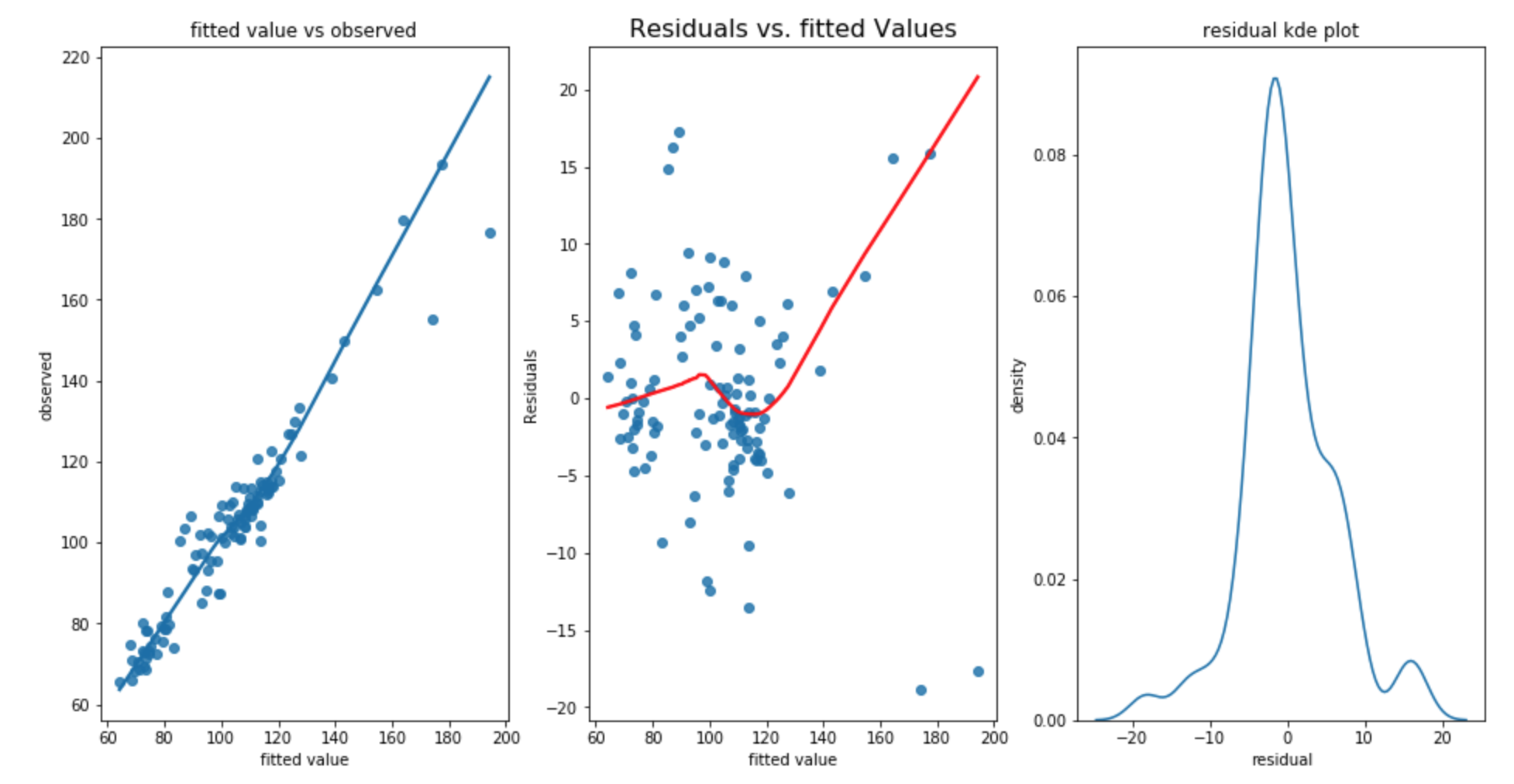
The above plot shows that

• the first plot shows that linearity appers to be satisfied.
• Bowl shaped curve in second graph shows the residual increases as fitted value increases. The homoscadacity is not met.
• the third graph shows that the there is a small second peak around 15 which shows that the normality assumption is not met.

2. square transform of dependent variable

   

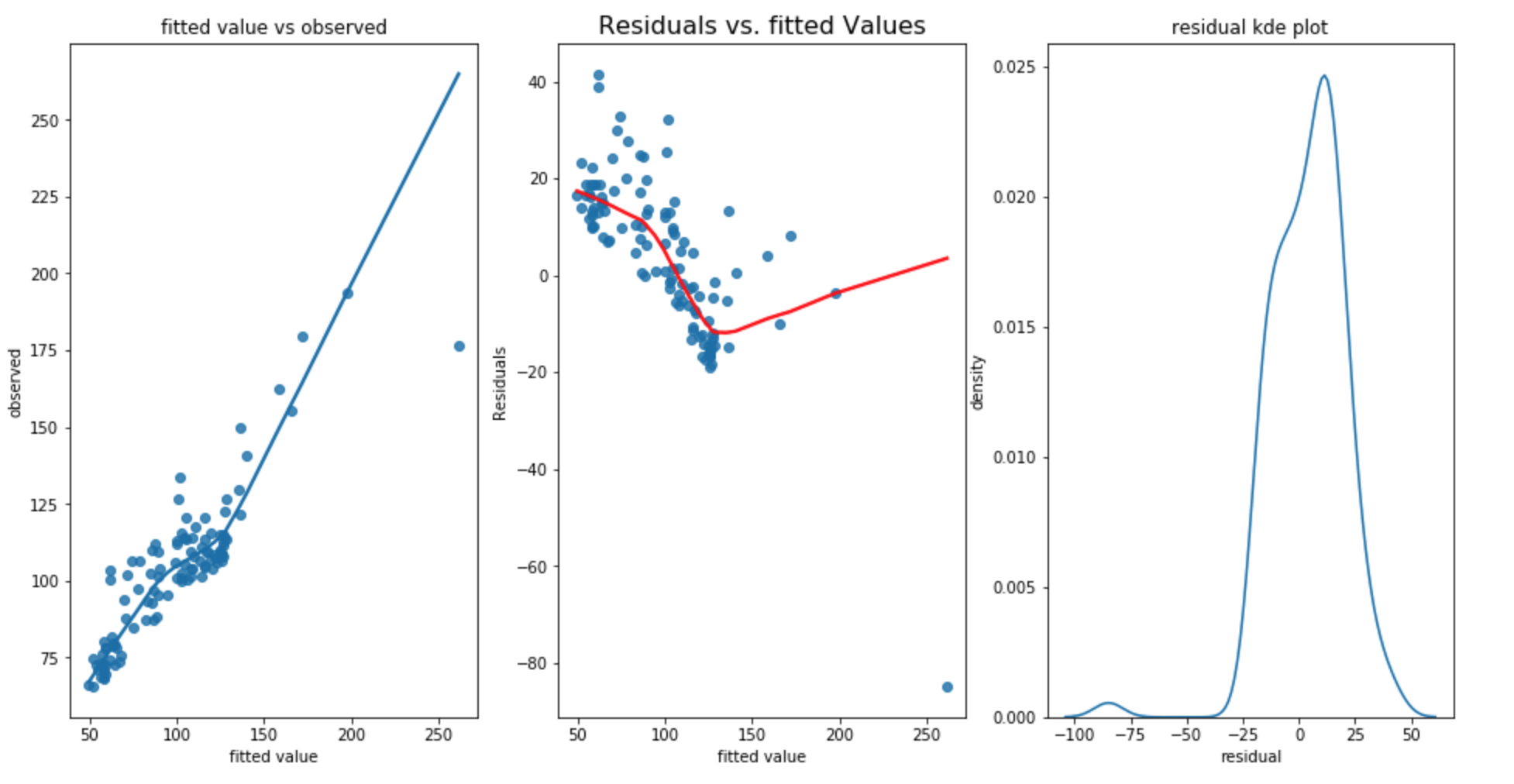
   From the above three graphs, it shows that there is no improvement on homoscedecity and the residual is not normal. In addition, RMSE for training dataset is 16.805, RMSE for test dataset is 9.085 and standard deviation of test dataset is 13.967 which shows that the training RMSE has increased and the test RMSE stays the same. The Durbain Watson statistic is 0.859 which shows more positive autocorrelation. It is not a good transformation.

3. add linear and quaratic term as independent variables

   2. a linear regression without trend term:

      $y_t = \beta_0 + \beta_1 * X + \epsilon$

      a linear regression with linear time trend:

      $y_t = \beta_0 + \beta_1 * X + \beta_2*t + \epsilon$

      where t represents the date, it can be encoded as 1, 2, 3 … so forth

      a linear regression with quadratic time trend:

      $y_t = \beta_0 + \beta_1 * X + \beta_2*t^2 + \epsilon$

      

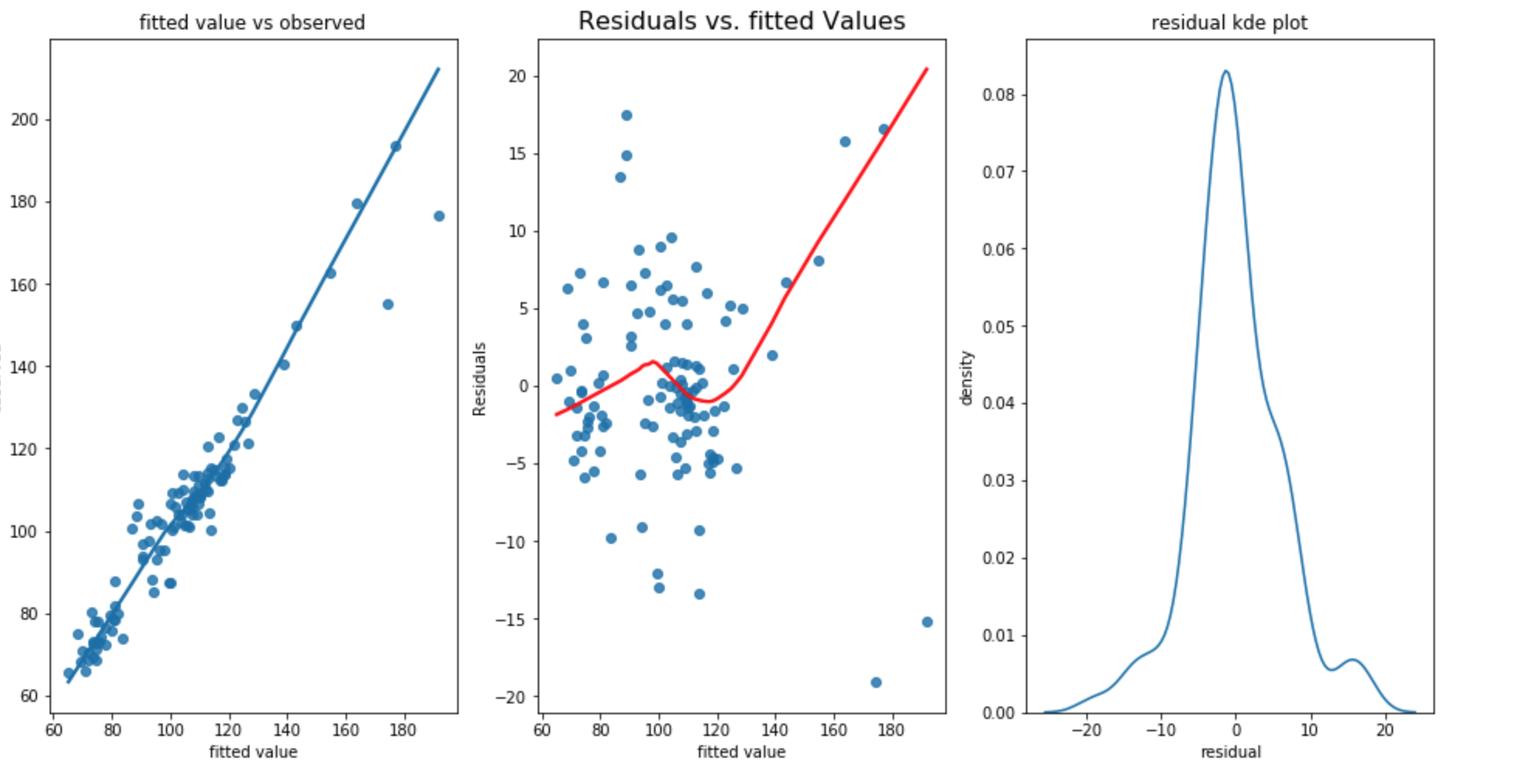
      RMSE for training dataset is 6.078, RMSE for test dataset is 9.781 and standard deviation of test dataset is 13.967. The result does not show significant improvement. However, the DW statistic is 1.59 which is worse then the first approach.

4. add extra features with lag = 2 with model expressed in the following equation:

   $y_t = \beta_0 + \beta_1 * x + \beta_2*y_{t-1} + \beta_3* x_{t-1} + \beta_4*y_{t-2}+\beta_5*x_{t-2} + \epsilon$

   

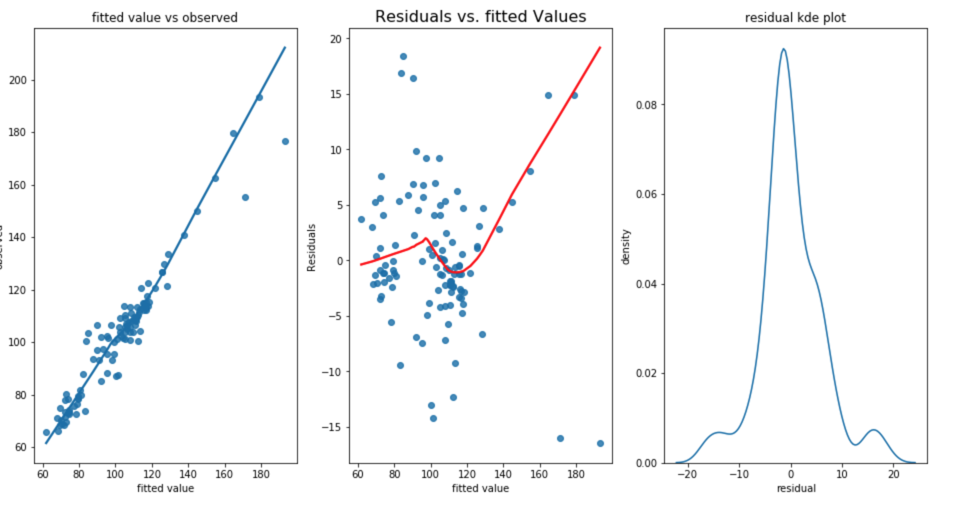
   RMSE for training dataset is 6.026, RMSE for test dataset is 7.200 and standard deviation of test dataset is 13.967. The Durbin Watson test statistic is 1.98 which shows there is not autocorrelation within the residual (better than first approach). However, the test RMSE is still not as good as first approach.

   put in a summary approach 1 (add extra feature with lag value = 1) appears to give the best performance based on RMSE and Durbain Watson statistics. Next, I would like to explore different models.

   model Selection with walk forward validation

   Since there is a singificant increasing/decreasing trend in the residual, I would like to try out gradient boosting models since it can learn the relationship between the input variable and the previous residual and Perhaps it may produce better result.

   from sklearn.model_selection import TimeSeriesSplit
   from sklearn.linear_model import LinearRegression
   def backtest(X,y,model,num_splits,metrics):
       '''splits dataframe into several fold with different variance and measure test metrics
       Parameters
       ----------
       X:input variables. Pandas.Series
       y:output variable. Pandas.Series
       model: the model you want to test. 
       splits: number of folds. float
       metrics: the metrics we want to measure rmse or mae
          
       Return
       ------
       table: each fold with test statistics
       '''
       splits = TimeSeriesSplit(num_splits)
       table = {}
          
       index = 1
       for train_idx, test_idx in splits.split(X):
           x_train, y_train = X[train_idx], y[train_idx]
           x_test, y_test = X[test_idx], y[test_idx]
      
           if model == 'linear_regression':
               model = LinearRegression()
           elif model == 'gradient_boosting':
               model = GradientBoostingRegressor()
           model.fit(x_train,y_train)
           y_pred = model.predict(x_test) 
           if metrics == 'rmse':
               measure_metric = np.sqrt(mean_squared_error(y_test,y_pred))
           elif metrics == 'mae':
               measure_metric = np.mean(np.abs(y_test-y_pred))
           test_std = np.std(y_test)
           train_rmse = np.sqrt(mean_squared_error(y_train,model.predict(x_train)))
      
           table['split'+str(index)] = [train_rmse,measure_metric,test_std]
           index += 1
       result = pd.DataFrame([(k,v[0],v[1],v[2]) for k,v in table.items()],columns=['fold','train_rmse',"test_"+metrics,'test standard deviation'])
       return result
   

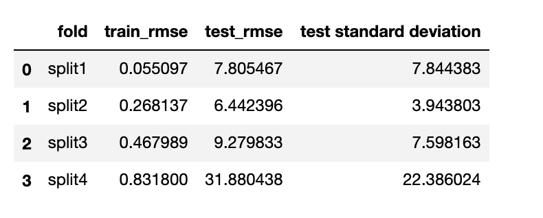
   walk forward validation with gradient boosting regressor:

   

   walk forward validation with linear regression:

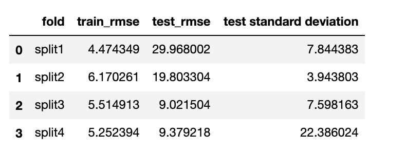   we can clearly see that gradient boosting regressor’s training_rmse is really small. However, the root mean squared error on test datase is approximatly 10-100 times of the training root mean squared error which shows that the algorithm is overfitting. On the other hand, linear regression algorithm is less overfitted when test with different dataset with different variance. It is more generalizable. Since we would like to predict a general trend of the house price index in next year. Linear regression model will be the most ideal.

   final model

   after running linear regression on dataset from 1890 until 2009. we have the following model

   

   The test RMSE is 9.085 and the test dataset standard deviation is 13.967.

   The significant indicator varaibles are

upsample dataset approach

The second method is upsampling the dataset from 1890 to 1952 from yearly bases to monthly bases. We will use the linear interpolation as default parameters.

from datetime import datetime, timedelta
def upsample(original_df,numDays='30D',method='pad'):
    '''the function is going to upsample the original dataframe by specific number of days
    Parameters
    ----------
    original_df: original dataframe. Pandas.dataframe
    numDays: number of days that I intend to upsampled
    method: the interpolate method can be 'linear','pad',
    
    Return
    ------
    df: new dataframe. Pandas.dataframe
    '''
    df = origin_df
    #split the data into two different dataframe with different sampling frequency
    df1 = df[df['home_index_date'] <= 1952]
    df2 = df[df['home_index_date'] > 1952]
    #convert the float date into datetime object
    df2['year'],df2['day_fraction'] = df['home_index_date'].divmod(1)
    df1['date'] = pd.to_datetime(df['home_index_date'].astype(int).astype(str),format='%Y')
    df1 = df1.drop('home_index_date',axis=1)
    df2['day'] = (365*df2['day_fraction']).astype(int)
    
    def convert_date(row):
        year = pd.to_datetime(row['year'],format='%Y')
        date = year + timedelta(row['day'])
        return date 
    df2['date'] = df2[['year','day']].apply(convert_date,axis=1)
    
    df2 = df2.drop(['home_index_date','year','day','day_fraction'],axis=1)
    df1.index = df1['date']
    df2.index = df2['date']
    #upsample the date with specific number of days
    upsampled = df1[['real_home_index','real_cost_index','population','long_rate','cpi_annual']].resample(numDays) 
    interpolated = upsampled.interpolate(method=method)
    df2 = df2.drop('date',axis=1)
    df = pd.concat([interpolated,df2],axis=0)
    df = df.reset_index()
    df = df.rename(columns={'date':'home_index_date'})
    
    return df

After upsampling the dataset, there are 1534 observations and the dataset looks like the below

I also decide to use the latest 10 years of data as test data. since the dataset is sampled on monthly bases. There will be total 120 observations in test dataset and the rest data as training dataset. SInce there are over 1000 features, I would like to add extra features with lag value of 1 and lag value of 2 to improve the RMSE statistics.

Lets the fit the linear regression model and check our residual

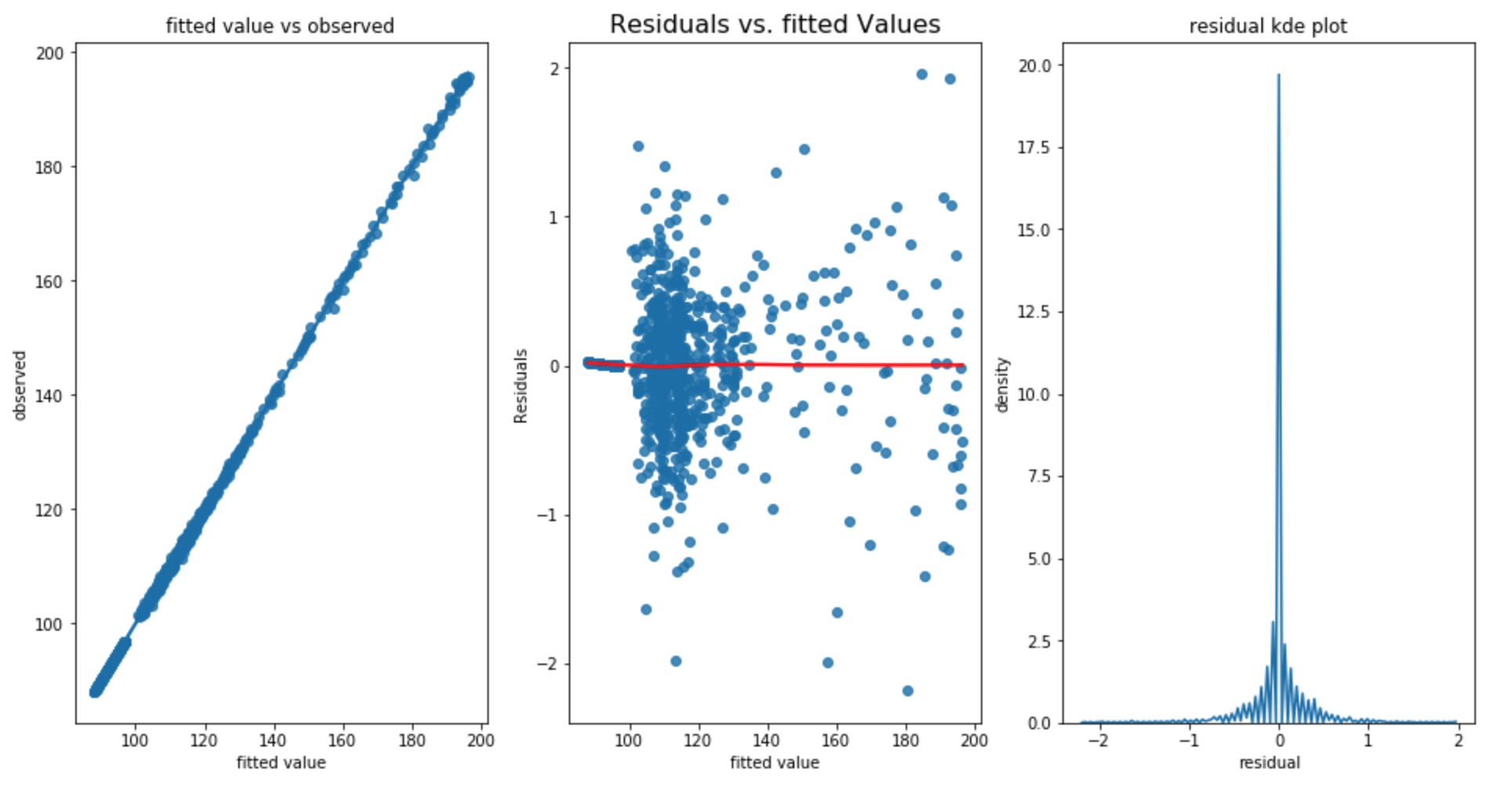
Wow, The R^2 value is almost 1 and the second plot also shows the homoscedacity assumption is met. However, the residual error appears to be not so normal. And the test_rmse is 0.724; train_rmse is 0.340, test dataset has standard deviation of 13.516 which shows that our model has improved significantly.

Since I am padding the dataset with linear interpolation and could potentially add extra noise in the dataset. I then decided to only use the dataset after 1953 to perform a linear regression and compare our result.

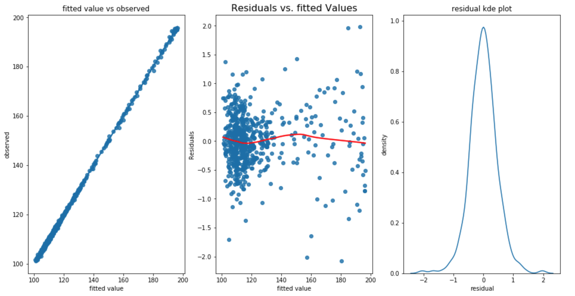
The testing RMSE is 0.682, the training RMSE is 0.462 and the test standard deviation is 13.516. From the above three plot, we can say that our linearity, homoscedacity, normality assumption has all met. In addition, the Durbin Watson statistic is 2.24 which shows that our residual has almost no autocorrelation.

The final model on monthly sampled dataset are expressed as following:

test final model on yearly based data

I would like to test our final model on the monthly sampled data and compare the result.

The RMSE for downsampling approach is 9.085 and the RMSE for upsampling approach is 7.779 and the standard deviation of test dataset is 13.967 which shows that our upsampling approach model performs better.

Interesting finding

• feature engineering with different time lags can significantly reduce the issue of residual autocorrelation
• In this dataset, log, square transform the dataset or add linear trend is not as useful as add lagged feature to reduce the autocorrelation within the dataset.
• Gradient boosting regressor is quite easy to overfit. Another challenge is to find the correct regulation parameters which takes more time to search. Thus, using Linear regression may be our best choice.
• On yearly based data, the significant indicator variables are real_home_index_lag_1, real_home_index_lag_2,
• on monthly based data, the significant indicator variables are cpi_annual,real_home_index_lag_1, long_rate_lag_1 cpi_annual_lag_1, real_home_index_lag_2
• upsample data with padding/linear increase tecnique has very little effect on getting better generality of the model. We cannot assume the fact that the house price, cost index, population, mogage rate, is neither constant nor in linear increasing pattern. In addition, padding also adds extra level of noise which may cause the model to mistaken the significance of an indicator varaible. We may be better off just use the original data.
• our model comparison has indicate that the regression model trained on monthly sampled dataset has achieved better RMSE score. higher sampling frequency can obtain more trend information in the market and with more data you can collect, the better result your model can offer.
• in both of our model, previous house index and previous two year house index has shown to be a significant variable and with a positive coefficient on previous year house index and negative coefficient on previous two year house index which shows that there may be some house price period cycle exist not only yearly but also monthly.

You can find my Jupyter notebook Here