Insect Image Recognition

With the dawn of a new era of A.I., machine learning, and robotics, its time for the machines to perform tasks characteristic of human intelligence.From Automated self-driven cars to Boosting augmented reality applications and gaming, from Image and Face Recognition on Social Networks to Its application in various Medical fields, Image Recognition has emerged as a powerful tool and has become a vital for many upcoming inventions.

Introduction

In this tutorial, we will present two effective methods to build a powerful insect image classifer. The idea is to create a simple, beetles, cockroaches, dragonflies image classifier and then comparing with existing benchmark models.

Collecting Dataset

The original dataset is found at the Insect Image websites. There are total 1199 images of beetles, cockroaches and dragonflies.

Image exploration

import matplotlib.image as mpimg
import matplotlib.pyplot as plt
beetle = mpimg.imread('train/beetles/5556579.jpg')
plt.imshow(beetle)

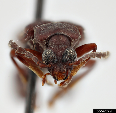
cockroach = mpimg.imread('train/cockroach/1233109.jpg')
plt.imshow(cockroach)

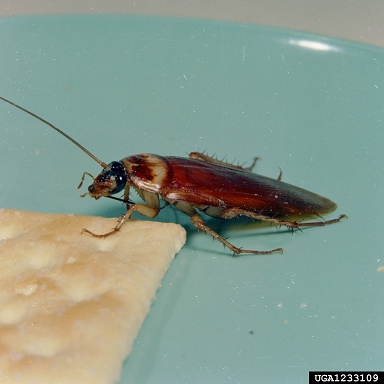
dragonfly = mpimg.imread('train/dragonflies/1113001.jpg')
plt.imshow(dragonfly)

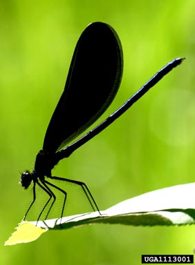
Load train and test dataset

After we download our train and test dataset, the images may not all consist in the exact pixel shapes. Thus, we have to resize each image into (64,64,3) (image height,imgae width,color channel) shape and stored all images as a numpy array.

def load_images(folder):
    '''load all images in current folder and return as a numpy array
    Parameters
    ----------
    folder: current directory. string
    
    Return
    ------
    imageArray: array of imgaes. numpy.array
    
    '''
    images = []
    for filename in os.listdir(folder):
        img = Image.open(os.path.join(folder, filename))
        #img = ImageOps.grayscale(img)
        if img is not None:
            image_resized = img_to_array(img.resize((64, 64)))
            images.append(image_resized)
    return np.array(images)

After load all the train and test images, we have 1109 training images and 180 testing images with shape (64,64,3)

Build Convolutional Neural network

This is most important step for our network. It consists of three parts -

1. Convolution

2. Pooling

3. Flattening

The primary purpose of Convolution is to extract features from the input image. Convolution preserves the spatial relationship between pixels by learning image features using small squares of input data.

Since every image can be considered as a matrix of pixel values. Consider a 5 x 5 image whose pixel values are only 0 and 1 (note that for a grayscale image, pixel values range from 0 to 255, the green matrix below is a special case where pixel values are only 0 and 1):

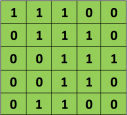
Also, consider another 3 x 3 matrix as shown below:

Then, the Convolution of the 5 x 5 image and the 3 x 3 matrix can be computed as shown in the animation in below:

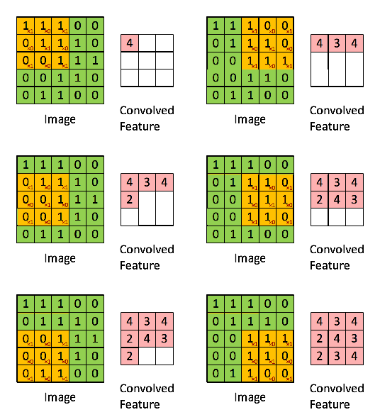
The obtained matrix is also known as the feature map. An additional operation called ReLU is used after every Convolution operation. The next step is of pooling.

Pooling (also called subsampling or downsampling) reduces the dimensionality of each feature map but retains the most important information. In case of Max Pooling, we define a spatial neighborhood (for example, a 2×2 window) and take the largest element from the rectified feature map within that window. Instead of taking the largest element we could also take the average (Average Pooling) or sum of all elements in that window. In practice, Max Pooling has been shown to work better.

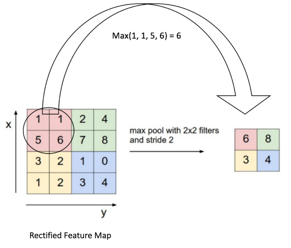
After pooling comes flattening. Here the matrix is converted into a linear array so that to input it into the nodes of our neural network.

Here is the code

def ImageModel(input_shape):
    # Define the input placeholder as a tensor with shape input_shape. Think of this as your input image!
    X_input = Input(input_shape)
    X = X_input

    # CONV -> BN -> RELU Block applied to X
    X = Conv2D(32, (4, 4), strides = (1, 1), name = 'conv0')(X)
    X = BatchNormalization(axis = 3, name = 'bn0')(X)
    X = Activation('relu')(X)

    # MAXPOOL
    X = MaxPooling2D((2, 2), name='max_pool1')(X)
    
    # CONV -> BN -> RELU Block applied to X
    X = Conv2D(64, (4, 4), strides = (1, 1), name = 'conv1')(X)
    X = BatchNormalization(axis = 3, name = 'bn1')(X)
    X = Activation('relu')(X)

    # MAXPOOL
    X = MaxPooling2D((2, 2), name='max_pool2')(X)

    # FLATTEN X (means convert it to a vector) + FULLYCONNECTED
    X = Flatten()(X)
    X = Dense(4, activation='softmax', name='fc')(X)

    # Create model. This creates your Keras model instance, you'll use this instance to train/test the model.
    model = Model(inputs = X_input, outputs = X, name='ImageModel')
    
    return model

So now our CNN network looks like this

Training the network

imageModel.fit(x=X_train, y=y_train, epochs=25, batch_size=64,shuffle=True,verbose=2)

So, we completed all the steps of construction and its time to train our model.

Testing the network

preds = imageModel.evaluate(x=X_test, y=y_test)
print()
print ("Loss = " + str(preds[0]))
print ("Test Accuracy = " + str(preds[1]))

our model has reached accuracy of 80%. Though it is not 100% accurate but it will give correct predictions most of the times. Try adding more convolutional and pooling layers, play with the number of nodes and epochs, and you might get high accuracy result.

Transfer Learning

we take the pre-trained weights of an already trained model(one that has been trained on millions of images belonging to 1000’s of classes, on several high power GPU’s for several days) and use these already learned features to predict new classes.

There are several models that have been trained on the image net dataset and have been open sourced.

For example, VGG-16, VGG-19, Inception-V3 etc. For more details about each of these models, read the official keras documentation here.

I decide to use VGG-19 in this example, code as following

base_model = VGG19(
    weights='imagenet', 
    include_top=False,
    input_shape=X_train.shape[1:],
    classes=3
)
x = base_model.output
x = GlobalAveragePooling2D()(x)
x = Dense(1024, activation='relu')(x)
output = Dense(4, activation='softmax')(x)
model = Model(inputs=base_model.input, outputs=output)
model.compile(
    optimizer='adam',
    loss='categorical_crossentropy',
    metrics=['accuracy']
)

The VGG-19 network looks like this

Testing network accuracy

model.fit(X_train,y_train, epochs=25,verbose=2,shuffle=True)
test_loss, test_acc = model.evaluate(X_test,y_test)
print(test_acc)

Our model has reach 100% accuracy! Even though it has reached high accuracy due to the limited sample of testing images.

Summary

So, we created a simple Image Recognition Classifier. The same concept can applied to a diverse range of objects with a lot of training data and appropriate network. You can change the dataset with the images of your friends and relatives and work upon the network to make a Face Recognition Classifier.