why forecast?
Becasue, forecasting a time series has tremendous value. In the ad analysis project, predicting the number of impression for different ads can drive a company’s decision on how to spend their money on ads.
Forecasting can be divided into two parts:
- Univeriate Time Series Forecasting: if you only use the previous value of a time series to predict the future value
- multivariate Time Series Forecasting: if you use external variables to forecast the future value.
1. Introdiction to ARIMA model
In this blog, I will particularly focus on ARIMA modeling which stands for “Auto Regressive Integrated Moving Average”, it is a univariate time series forecasting algorithm that can be used to predict the future value.
An ARIMA model can be characterized by three terms: p, d, q where
p is the order of AR term
q is the order of MA term
d is the number of the differencing that can make the time series stationary.
How to build ARIMA model?
- make the time series staionary
- determine the optimal p,d,q term
- Forecast the residual and take it back to original scale
- evaluete the final model
2. why stationary?
because ARIMA model is a specialized Linear Rgression model that uses its own lags as predictors. One of the requirement for linear regression is to ensure that their predictor is independent.
how to make stationary
- exponential smoothing
- differencing
- decomposing
3. What are AR and MA models
AR stands for autoregressive model which means the target variable only depends on its preivous lagged value. It can be expressed as following equation (error is irreducible)
$Y_t = \alpha + \beta_1*Y_{t-1} + \beta_2*Y_{t-2} + ….. +error $
MA stands for moving average model which means taht the target variable depends on a lagged forecast error . it can be expressed as following equation ($\epsilon_t$ is irreducible)
$Y_t = \mu + \phi_1 * \epsilon_{t-1} + \phi_2 * \epsilon_{t-2} + …. + \epsilon_t$
ARIMA model is a combination of AR and MA terms. It can be expressed as the following equation:
$Y_t = \alpha + \beta_1*Y_{t-1} + \beta_2*Y_{t-2} +\beta_3 * \epsilon_{t-1} + \beta_4* \epsilon_{t-2} + ….. $
4. how to determine the p term
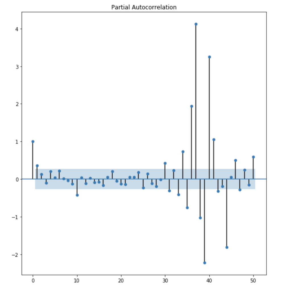
the p term can be identified by inspecting the PACF(partial autocorrelation) plot
what is PACF plot ?
looking at the AR term, the partial autocorrealtion are the correlation between the series and its lagged value. After excluding the contribution from the intermediate value. The PACF express the direct correlation between value and lags.
Determine the p term based on PACF plot:

The shaded area within the graph is considered as confidence interval suggest that the correlation values outside of this band are likely a correaltion and not a statistical fluke. From the above plot, we can observe that lag 1 is quite significant since it is well above the confidence interval band. lag 2 is significant as well. However, I am going to be conservative and choose the p term to be 1.
5. How to determine the q term
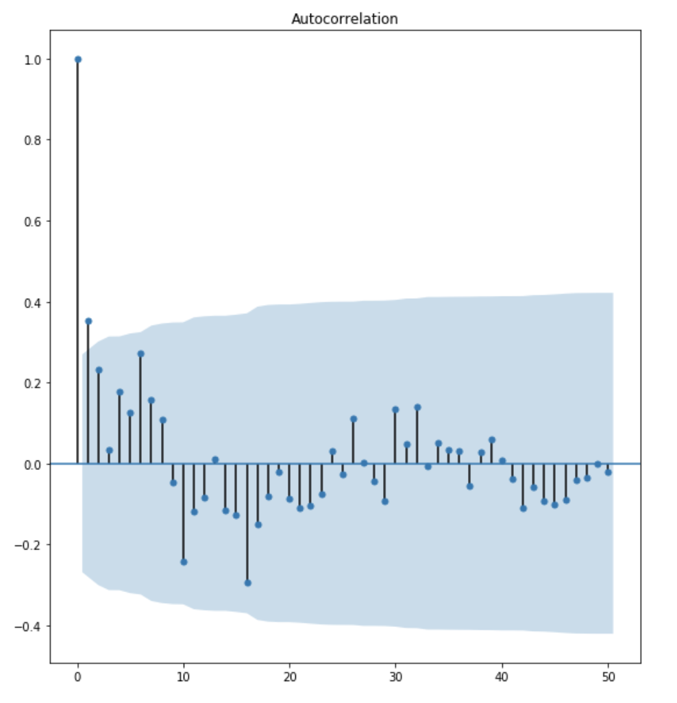
the q term can be identified by inspecting the ACF (Autocorrelation) plot.
what is ACF plot?
The ACF plot tells how many MA terms are required to remove any autocorrelation in the stationary series.
Determine the q term based on ACF plot:

The inspection process are similar to the inspection process for PACF plot. The above plot shows that lag 1 and lag 2 are significant. I am going to be conservative and choose the q term to be 1.
6. How to determine the d term
the objective of differencing is to make the time series stationary. It is also important to not over difference the time series. if you can’t decide between two order of differecing, then go with the order that gives less standard deviation
determine the d term based on ndiff from arima.utils
from pmdarima.arima.utils import ndiffs
df = pd.read_csv('file_name')
y = df.values
ndiffs(y, test='adf')
the program above will perform a test of stationarity for different level of d to estimate the number of difference required to make a given time series stationary. it will select the maximum value of d term for which the time series is judged stationary by the statistical test.
7. How to build ARMA model
Now lets use the ARIMA mdoel from statsmodels package. Since the dataset that I use is stationary. I will build ARMA model here. The process is similar.
model = ARIMA(ad_group['shown'],order=(1,0,2))
final_ARMA = model.fit(disp=0)
print(final_ARMA.summary())

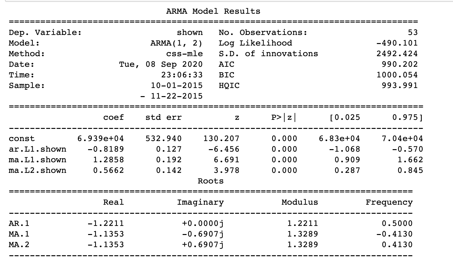
The model summary reveals a lot of imformation. the coefficients are the weights for each lagged term and the p >|z| are the p-value for the coefficients. it should ideally less then 0.05 for the input variable to be significant.
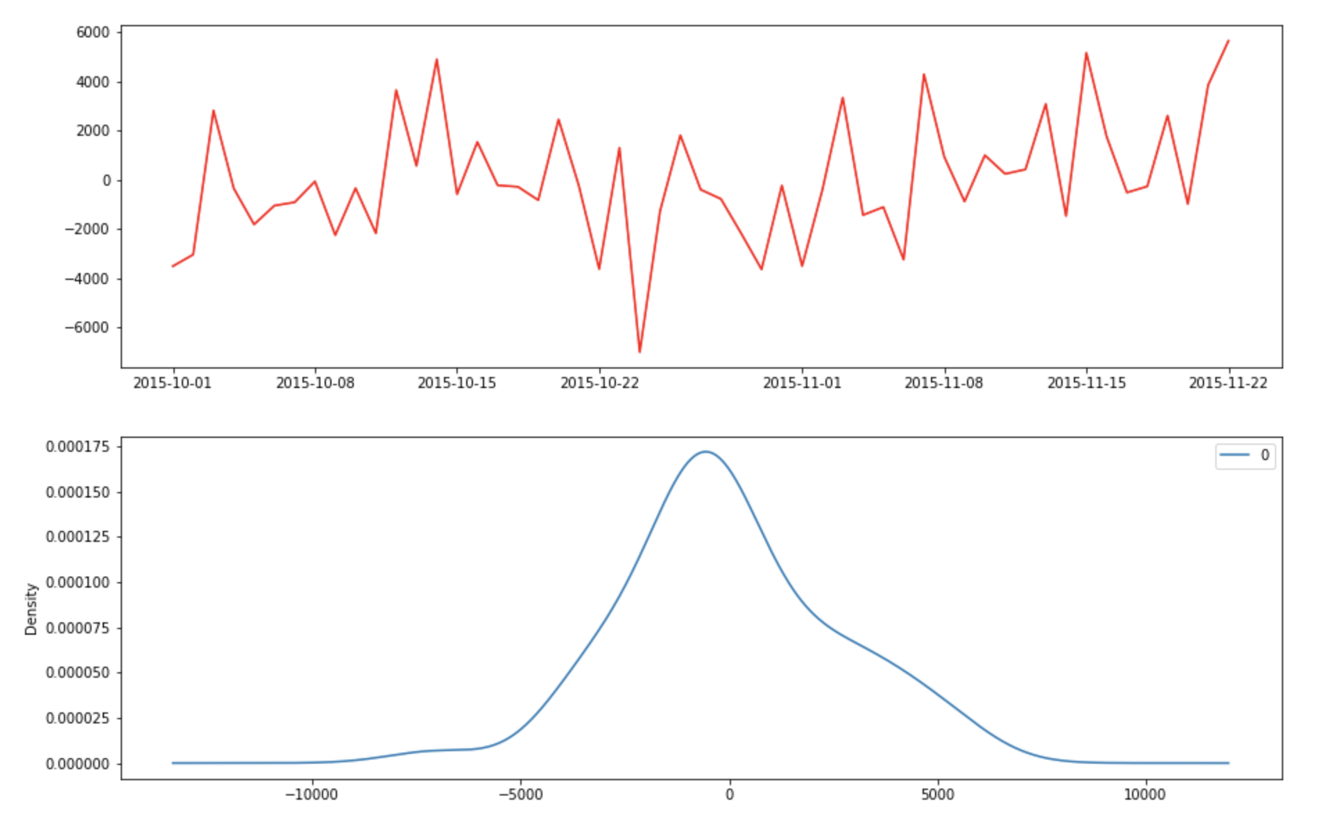
It is also important to plot the residual to ensure that there is not pattern (look for constant mean and variance)
fig, axes = plt.subplots(2,1,figsize=(15,10))
axes[0].plot(ad_group)
axes[0].plot(final_ARMA.fittedvalues, color='red')
residuals = pd.DataFrame(final_ARMA.resid)
residuals.plot(kind='kde',ax=axes[1])

The residual errors appears to have 0 mean and constant variance. Let’s plot true Xagainst the fitted values.

The result looks decent. However, we can still do it better by perform grid. search for our model.
def grid_search_arima(data):
    mat_aic = np.zeros((5,5))
    for p in range(1,6):
        for q in range(1,6):
            try:
                #build model for each p,q
                model = ARIMA(data,order=(p,0,q))
                results_ARMA = model.fit(disp=0)
                #fill mat_aic with corresponding p,q
                mat_aic[p-1][q-1] = results_ARMA.aic
            except:
                print('not invertible')
    #print(mat_aic)
    min_i, min_j = None, None
    min_aic = float('inf')
    #find the index of minimum aic score in mat_aic
    for i in range(mat_aic.shape[0]):
        for j in range(mat_aic.shape[1]):
            if mat_aic[i][j] < min_aic and mat_aic[i][j] != 0:
                min_aic = mat_aic[i][j]
                min_i, min_j = i,j
    return min_i + 1, min_j + 1
The metrics that we use to evaluate ARMA model is AIC score. AIC (Akaike information crieterion) score is an estimator of out-of-sample prediction error and a relative quality of statistical model for a given set of data. It is a relative score and it is only useful when comparing with other model’s AIC score.
AIC works by evaluating the models’ fit on the training data and adding a penalty term for the complexity of the model. The desired result is to find the lowest possible AIC which indicates the best balance of model fit with generalizability.
AIC uses the model’s maximum likelihood estimation as a measure of fit. The model that gives the maximum likelihood of the observed data is the best ‘fit’ data. AIC is low when the likelihood are high. There are also assumptions to use AIC score:
- using the same dataset between model
- measure the same outcome variable between model
8. How to evalute ARIMA model with walk forward validation
In general machine learning, we would like to use cross validation for our machine learning model. However, the issue with cross validation is that when we are partitioning the training data into each fold, we are randomly select samples which means that we have dirupt the temporal order of the dataset. the test dataset may not contain the latest data. The information leakage is a problem that we need to solve.
Walk forward validation requires multiple models to be trained and evaluated. It helps to preserve the temporal order of the dataset. we have to make two decision:
- Minimum number of observation. First, we must select the minimum number of observations required to train the model.
- Sliding or expanding window: we need to decide how many new data are we going to include each time we are going to retrain the model.
- start at the begnning of the time series, the minimum number of observation is used to train a model.
- the model makes prediction for the next time step
- the prediction is stored and evaluate against the known value.
- the window is expanded to include the known value and retrain the new model (repeat step 1)
In the scikit-learn package, there is a TimeSeriesSplit object which can help us illustrate this validation
The total number of training and testing observations are calculated at each iteration i:
training_size = i * n_samples // (n_splits + 1) + n_samples % (n_splits + 1)
test_size = n_samples//(n_splits + 1)
where n_samples is the total number of observations And n_splits is the total number of splits. The dataset has 174 observations and I decide to create 4 splits, using the algorithm above, we can expected the following train and test set to be created:
- Split1: 38 train, 34 test
- Split2: 72 train, 34 test
- Split3: 106train, 34test
- Split4 : 140train, 34 test
As you can see that the model has trained on larger and larger history. This is interesting becuse at different time interval, the variance of the data are different. It provides a better picture of how generalized the model is. In addition, the test size stays consistent which means we can compare each split’s result. In the example below, I choose the Root mean squared error as a metric to evalute the model peformance.
def backtest_model(data,model,split):
    if isinstance(data,pd.DataFrame):
        X = data.values
    else:
        X = data
    splits_rmse = []
    splits = TimeSeriesSplit(split)
    for train_index, test_index in splits.split(X):
        train = X[train_index]
        test = X[test_index]
        period = len(test)
        predict = np.zeros(test.shape)
        forecast,_,_ = model.forecast(steps=period,alpha=0.05)
        rmse = math.sqrt(mean_squared_error(test,forecast))
        splits_rmse.append(rmse)
    return splits_rmse
After running the above program. the average root mean squared error (standard deviation of prediction error) of four splits is 2887 and the standard deviation of the dataset is 2830 which means that our model prediction is quite good.
9. accuracy metrics for time series forecast
- Mean Absolute Percentage Error (MAPE)
- Mean Error (ME)
- Mean Absolute Error (MAE)
- Mean Percentage Error (MPE)
- Root Mean Squared Error (RMSE)
The MAPE are more commonly used to forecast two different series since it is a percentage error which vary between 0 and 1. You can judge the forecast disregard the scale of the time series.
The other metrics are quantitative metrics which can be hard to compare the forecast of two different scaled time series.